Exchange Traded Funds
A collection of securities for example stocks which usually tracks an underlying index is known as an Exchange - Traded Fund(ETF). ETF’s share some similarity with mutual funds although they are listed on exchanges and their share is traded like stocks throughout the day. ETF’s can be made up of various strategies and invest in diverse number of industry sectors.
The most popular index tracked by most ETF’s is the S&P 500. For example the SPDR S&P 500 ETF (SPY) tracks the S&P 500. ETFs can include different types of investments, including stocks, commodities, bonds, or a mixture of investment types. ETF’s is traded on financial markets as a security with a price at which it can be bought and sold. Most ETF’s are set up as Open-end funds meaning there is no cap on the number of investors allowed in on the product.
Types of ETFs
There are various types of ETFs available to investors that can be used for income generation, speculation, price increases, and to hedge or partly offset risk in an investor’s portfolio. Below are several examples of the types of ETFs.
- Bond ETFs may include government bonds, corporate bonds, and state and local government bonds called municipal bonds.
- Industry ETFs track a particular industry such as technology, banking, or the oil and gas sector.
- Commodity ETFs invest in commodities including crude oil or gold.
- Currency ETFs invest in foreign currencies such as the Euro or the British pound.
- Inverse ETFs attempt to earn gains from stock declines by shorting stocks. Shorting is selling a stock, expecting a decline in value, and repurchasing it at a lower price. Many inverse ETFs are Exchange Traded Notes (ETNs) and not true ETFs. An ETN is a bond but trades like a stock and is backed by an issuer like a bank.
How to Buy and Sell ETFs
ETF’s are traded through licensed online and traditional broker dealers. Most of the poular ETF brokers like Vanguard also have robo-advisors which is a computer algorithm that attempts to mimic a human trader. Some ETF’s go a step further by offering commision free products. Examples of such brokers can easily be found online.
The following libraries required is loaded loaded here.
library(ggplot2)
library(plotly)
library(rvest)
library(pbapply)
library(TTR)
library(dygraphs)
library(lubridate)
library(tidyquant)
library(timetk)
library(htmlwidgets)
library(kableExtra)
pacman::p_load(kable,dygraphs,DT,tidyverse,janitor,ggthemes,scales,ggpubr,viridis)

theme_set(theme_pubclean())
The table below shows some popular U.S. ETF brands and issuers.
library(rvest)
library(XML)
library(gt)
library(tidyverse)
library(glue)


webpage <- read_html("https://www.etf.com/sections/etf-league-tables/etf-league-table-2020-02-10")

tbls <- html_nodes(webpage, "table")

print(head(tbls))
## {xml_nodeset (2)}
## [1] <table border="0" cellpadding="2" cellspacing="0" class="IUtable" style=" ...
## [2] <table border="0" cellpadding="2" cellspacing="0" class="IUtable" style=" ...
tbls_ls <- webpage %>%
        html_nodes("table") %>%
        .[[1]] %>%
        html_table(fill = TRUE)


colnames(tbls_ls)  <-  c("Brand","AUM ($, mm)","Net Flows ($, mm)","% of AUM")

tbls_ls  <- tbls_ls %>% janitor::clean_names()


#DT::datatable(tbls_ls, class = 'cell-border stripe')

tbls_ls %>%head()%>%
  kable(escape = F, align = "c") %>%
  kable_styling(c("striped", "condensed"), full_width = F)
| brand | aum_mm | net_flows_mm | percent_of_aum |
|---|---|---|---|
| Brand | AUM ($, mm) | Net Flows ($, mm) | % of AUM |
| iShares | 1,761,739.92 | 1,120.23 | 0.06% |
| Vanguard | 1,195,773.48 | 1,154.64 | 0.10% |
| SPDR | 737,904.99 | -710.71 | -0.10% |
| Invesco | 232,732.50 | 250.17 | 0.11% |
| Schwab | 168,568.37 | 165.32 | 0.10% |
We can download the following ETF’s some of which are actively managed and others which are passively managed from the yahoo API using the quantmod API.
#library("RSelenium")

tickers= c("QQQ","IVV","SPY","VOO","VTI","IWB","GLD","EEM","XLF",
           "GDX","ARKW")

actively_managed =c("ARKW")

passively_managed <-  c("AGZ","IHI","IEUS","FCOM","VGT.IV","
VUG.IV")

vanguard <- c("MGK.IV","MGC.IV","VGT.IV","
VUG.IV","VONG.IV")

# The symbols vector holds our tickers.
symbols <- c("SPY","EFA", "IJS", "EEM","AGG")

# The prices object will hold our raw price data
prices <-
  quantmod::getSymbols(tickers, src = 'yahoo', from = "2010-01-01",
             auto.assign = TRUE, warnings = FALSE) %>%
 furrr::future_map(~Ad(get(.))) %>%
  reduce(merge) %>%   #reduce() combines from the left, reduce_right() combines from the right
  `colnames<-`(tickers)


#DT::datatable(data.frame(head(prices)))

data.frame(head(prices)) %>%head()%>%
  kable(escape = F, align = "c") %>%
  kable_styling(c("striped", "condensed"), full_width = F)
| QQQ | IVV | SPY | VOO | VTI | IWB | GLD | EEM | XLF | GDX | ARKW | |
|---|---|---|---|---|---|---|---|---|---|---|---|
| 2010-01-04 | 41.71869 | 92.10523 | 92.24605 | NA | 46.96941 | 51.31325 | 109.80 | 34.66187 | 7.660890 | 44.59262 | NA |
| 2010-01-05 | 41.71869 | 92.37265 | 92.49020 | NA | 47.14971 | 51.47793 | 109.70 | 34.91345 | 7.801696 | 45.02256 | NA |
| 2010-01-06 | 41.46705 | 92.44558 | 92.55533 | NA | 47.21528 | 51.54378 | 111.51 | 34.98648 | 7.817341 | 46.11611 | NA |
| 2010-01-07 | 41.49401 | 92.85078 | 92.94606 | NA | 47.41198 | 51.74965 | 110.82 | 34.78360 | 7.984223 | 45.89180 | NA |
| 2010-01-08 | 41.83553 | 93.16687 | 93.25535 | NA | 47.56769 | 51.92256 | 111.37 | 35.05952 | 7.937286 | 46.58344 | NA |
| 2010-01-11 | 41.66477 | 93.29655 | 93.38558 | NA | 47.63326 | 51.99666 | 112.85 | 34.98648 | 7.942502 | 46.89188 | NA |
The prices of these ETF’s can be visualized with dygraph package, it allows a user to set a date window which lets you expand and narrow the windows to focus on detail visualization within the range of interest.
dateWindow <- c("2015-01-01", "2020-02-20")

p1= dygraph(prices, main = "Value", group = "stock",
        xlab = "Time",ylab = "Adjusted Prices") %>%
  dyRebase(value = 100) %>%
  dyRangeSelector(dateWindow = dateWindow)


htmlwidgets::saveWidget(as_widget(p1), "p1.html")

p1
Convert daily prices to monthly prices using a call to to.monthly(prices, indexAt = “last”, OHLC = FALSE) from quantmod. The argument index = “last” tells the function whether we want to index to the first day of the month or the last day.
prices_monthly <- to.monthly(prices, indexAt = "last", OHLC = FALSE)%>%tk_tbl()%>% rename(date=index)


start_date <-first(index(prices_monthly))
end_date <- last(index(prices_monthly))

#prices_monthly  %>% head()   %>%  gt() %>%
#  tab_header(
#    title = " Monthly Prices for ETF's",
#    subtitle = glue::glue("{start_date} to {end_date}")
#  )


prices_monthly  %>% head()%>%
  kable(escape = F, align = "c") %>%
  kable_styling(c("striped", "condensed"), full_width = F)
| date | QQQ | IVV | SPY | VOO | VTI | IWB | GLD | EEM | XLF | GDX | ARKW |
|---|---|---|---|---|---|---|---|---|---|---|---|
| 2014-09-30 | 93.71915 | 176.6444 | 176.5203 | 161.6403 | 91.02445 | 98.94495 | 116.21 | 36.63364 | 12.99660 | 20.55621 | 16.92123 |
| 2014-10-31 | 96.19518 | 180.8587 | 180.6775 | 165.5249 | 93.52393 | 101.31341 | 112.66 | 37.15370 | 13.37242 | 16.56238 | 17.20904 |
| 2014-11-28 | 100.56856 | 185.8393 | 185.6411 | 170.0898 | 95.84360 | 104.06014 | 112.11 | 36.58075 | 13.68653 | 17.66910 | 17.52985 |
| 2014-12-31 | 98.31519 | 185.2874 | 185.1702 | 169.5703 | 95.80689 | 103.75922 | 113.58 | 35.13086 | 13.94251 | 17.80461 | 17.37833 |
| 2015-01-30 | 96.26794 | 179.9134 | 179.6837 | 164.7011 | 93.18576 | 100.97132 | 123.45 | 34.88944 | 12.97279 | 21.59221 | 17.32754 |
| 2015-02-27 | 103.21903 | 190.0703 | 189.7828 | 173.8906 | 98.53648 | 106.68292 | 116.16 | 36.42736 | 13.72827 | 20.61383 | 18.75810 |
We now have an xts object, and we have moved from daily prices to monthly prices.
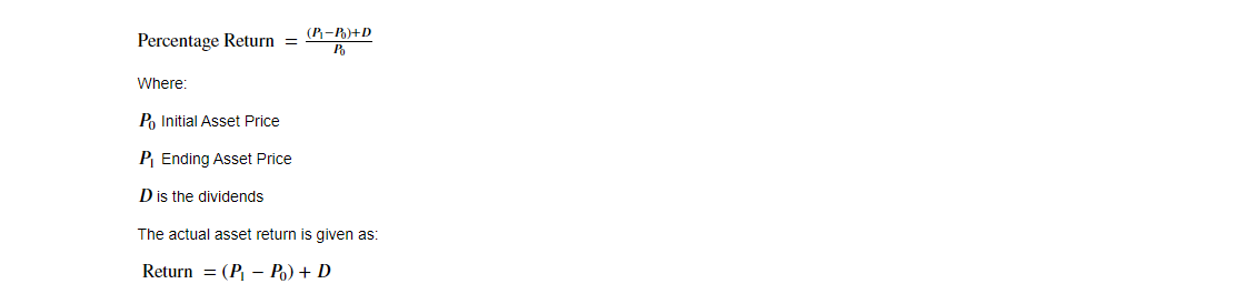
Return.calculate(prices_monthly, method = “log”) to convert to returns and save as an object called assed_returns_xts. Note this will give us log returns by the method = “log” argument. We could have used method = “discrete” to get simple returns. The daily percentage return on a stock is the difference between the previous day’s price and the current day’s price relative to the previous day’s price. The monthly perentage return follows as the difference between the previous month and the current month’s price divided by the previous months price.
#asset_returns_xts <- na.omit(Return.calculate(prices_monthly, method = "discreet"))
prices_monthly <- to.monthly(prices, indexAt = "last", OHLC = FALSE)
asset_returns_quantmod <- na.omit(CalculateReturns(prices_monthly, method = "log"))
head(asset_returns_quantmod)%>%tk_tbl()%>%
  kable(escape = F, align = "c") %>%
  kable_styling(c("striped", "condensed"), full_width = F)
| index | QQQ | IVV | SPY | VOO | VTI | IWB | GLD | EEM | XLF | GDX | ARKW |
|---|---|---|---|---|---|---|---|---|---|---|---|
| 2014-10-31 | 0.0260767 | 0.0235776 | 0.0232774 | 0.0237483 | 0.0270893 | 0.0236552 | -0.0310244 | 0.0140965 | 0.0285065 | -0.2160296 | 0.0168654 |
| 2014-11-28 | 0.0444605 | 0.0271660 | 0.0271016 | 0.0272043 | 0.0245003 | 0.0267502 | -0.0048939 | -0.0155414 | 0.0232182 | 0.0646838 | 0.0184708 |
| 2014-12-31 | -0.0226612 | -0.0029742 | -0.0025398 | -0.0030584 | -0.0003830 | -0.0028959 | 0.0130269 | -0.0404422 | 0.0185299 | 0.0076400 | -0.0086811 |
| 2015-01-30 | -0.0210432 | -0.0294324 | -0.0300770 | -0.0291356 | -0.0277397 | -0.0272365 | 0.0833287 | -0.0068957 | -0.0720882 | 0.1928753 | -0.0029269 |
| 2015-02-27 | 0.0697179 | 0.0549183 | 0.0546819 | 0.0542943 | 0.0558319 | 0.0550246 | -0.0608676 | 0.0431361 | 0.0566029 | -0.0463706 | 0.0793286 |
| 2015-03-31 | -0.0238725 | -0.0160997 | -0.0158302 | -0.0158327 | -0.0116970 | -0.0131021 | -0.0217570 | -0.0150863 | -0.0061797 | -0.1541505 | -0.0067920 |
pacman::p_load(kable,kableExtra)

ETF_returns <- prices %>%
  tk_tbl(preserve_index = TRUE, rename_index = "date") %>%

  pivot_longer(-date , names_to = "symbol",values_to = "Adjusted_Prices")%>%

  group_by(symbol) %>%
  tq_transmute(mutate_fun = periodReturn, period = "monthly", type = "log") %>%

  arrange(desc(monthly.returns))


ETF_returns%>%head()%>%
  kable(escape = F, align = "c") %>%
  kable_styling(c("striped", "condensed"), full_width = F)
| symbol | date | monthly.returns |
|---|---|---|
| GDX | 2020-04-30 | 0.3365961 |
| GDX | 2016-02-29 | 0.3102956 |
| GDX | 2016-04-29 | 0.2573056 |
| XLF | 2016-09-30 | 0.2350068 |
| ARKW | 2020-04-30 | 0.2197622 |
| GDX | 2016-06-30 | 0.2047288 |
An interactive visualiation for the monthly returns for the ETF’s selected is displayed below.
library(crosstalk)

ETF_returns <-  ETF_returns %>%  ungroup(symbol)


d <-
  SharedData$new(ETF_returns, ~symbol)
p2 <- ggplot(d, aes(date,monthly.returns,color=symbol)) +
  geom_line(aes(group = symbol))+


#scale_y_continuous(trans = log10_trans(), labels =  scales::comma)+

  #scale_fill_viridis_d()+
  scale_color_viridis_d(option="D") +

  # scale_shape_manual(values = 1:6 )  +

 #   theme_economist() +

  scale_x_date(labels = date_format("%d-%m-%Y"),date_breaks = "1 year") +
  theme(axis.text.x=element_text(angle=45, hjust=1)) +
   labs(title = "Monthly Returns Performance of Exhcange Traded Funds",
       subtitle = " 2010 - 2020",
       caption = "www.restsanalytics.com",
       x = "Time", y = "Returns")


(gg <- ggplotly(p2, tooltip = "symbol"))
gg=highlight(gg, "plotly_hover")
ggsave("p2.png")

#htmlwidgets::saveWidget(as_widget(gg), "p2.html")
htmlwidgets::saveWidget(gg, "p2.html", selfcontained = F, libdir = "lib")
#saveWidget(gg, file="p2.html")
gg
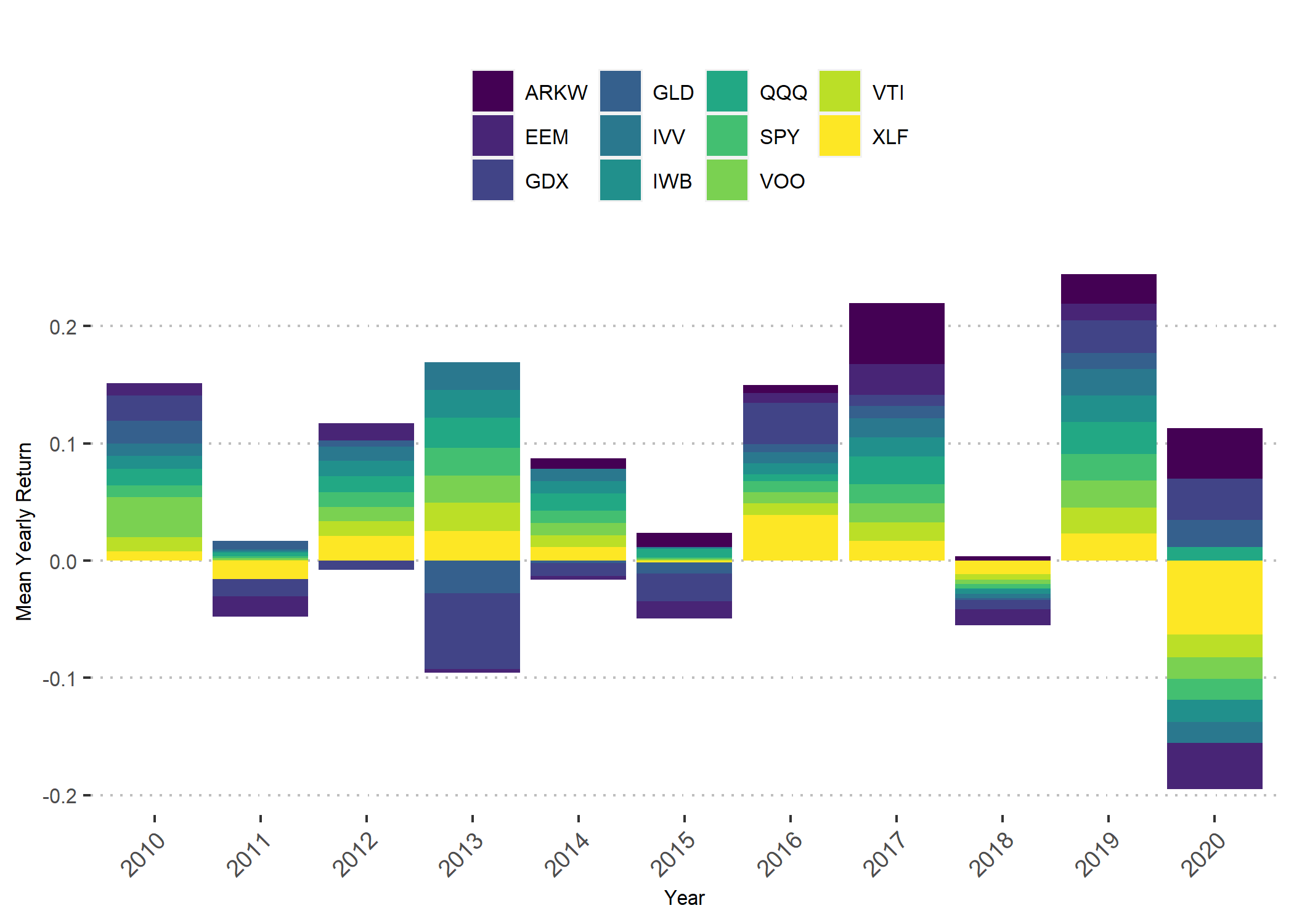
ETF_returns %>% mutate(Year= format(date,"%Y")) %>%  group_by(symbol,Year) %>%
                summarize(meanreturn =mean(monthly.returns,na.rm = TRUE))%>%

  ggplot(aes(x=Year,y=meanreturn,fill=symbol))+
  geom_col()+
 #scale_color_viridis(discrete=TRUE,option = "A")
scale_fill_viridis(discrete=TRUE,option = "D")+
    theme(
    legend.position="top",
    legend.direction="horizontal",
    legend.title = element_blank(),
    text=element_text(size=8,  family="Comic Sans MS"),
    axis.text.x=element_text(angle=45,hjust=1,size = 9),
    axis.text.y=element_text(size = 8),
    legend.text = element_text(size=8)
)+
   labs(y="Mean Yearly Return",x="Year",title="")
# scale_x_date(breaks = date_breaks("1 year"),labels=date_format("%b %Y") )
The analysis above in which the data was downloaded with the quantmod package, can be replicated with the tidyquant package. The tidyquant package builds a wrapper around the quantmod and converts the data from xts format to tibble dataframes.
end<-Sys.Date()
start<-as.Date("2010-01-10")


Prices  <- tq_get(tickers , get = "stock.prices", from = start,to=end)
#Prices%>%head() %>% DT::datatable()

Prices%>%head() %>%tk_tbl()%>%
  kable(escape = F, align = "c") %>%
  kable_styling(c("striped", "condensed"), full_width = F)
| symbol | date | open | high | low | close | volume | adjusted |
|---|---|---|---|---|---|---|---|
| QQQ | 2010-01-11 | 46.61 | 46.64 | 46.12 | 46.36 | 104673400 | 41.66477 |
| QQQ | 2010-01-12 | 46.08 | 46.14 | 45.53 | 45.78 | 90673900 | 41.14353 |
| QQQ | 2010-01-13 | 45.92 | 46.49 | 45.61 | 46.35 | 100661000 | 41.65579 |
| QQQ | 2010-01-14 | 46.26 | 46.52 | 46.22 | 46.39 | 75209000 | 41.69173 |
| QQQ | 2010-01-15 | 46.47 | 46.55 | 45.65 | 45.85 | 126849300 | 41.20641 |
| QQQ | 2010-01-19 | 45.96 | 46.64 | 45.95 | 46.59 | 84388200 | 41.87149 |
library(crosstalk)
d <- SharedData$new(Prices, ~symbol)
p3 <- ggplot(d, aes(date, adjusted,color=symbol)) +
  geom_line(aes(group = symbol))+


#scale_y_continuous(trans = log10_trans(), labels =  scales::comma)+

  #scale_fill_viridis_d()+
  scale_color_viridis_d(option="D") +

  # scale_shape_manual(values = 1:6 )  +

 #   theme_economist() +

  scale_x_date(labels = date_format("%d-%m-%Y"),date_breaks = "1 year") +
  theme(axis.text.x=element_text(angle=45, hjust=1)) +
   labs(title = "Performance of Exhcange Traded Funds",
       subtitle = " 2010 - 2020",
       caption = "www.restsanalytics.com",
       x = "Time", y = "Adjusted Prices")


(gg <- ggplotly(p3, tooltip = "symbol"))
gg=highlight(gg, "plotly_hover")


ggsave("p3.png")


htmlwidgets::saveWidget(as_widget(gg), "p3.html")
#htmlwidgets::saveWidget(gg, "p3.html", selfcontained = F, libdir = "lib")
gg
Returns
monthlyreturns <-Prices%>% select(symbol,date,adjusted)%>%
  group_by(symbol)%>%
  tq_transmute(
                 mutate_fun = periodReturn,
                 period     = "monthly",
                 type       = "arithmetic")%>%head()


#monthlyreturns%>%head() %>% gt()

monthlyreturns%>%head()  %>%tk_tbl()%>%
  kable(escape = F, align = "c") %>%
  kable_styling(c("striped", "condensed"), full_width = F)
| symbol | date | monthly.returns |
|---|---|---|
| QQQ | 2010-01-29 | -0.0770059 |
| QQQ | 2010-02-26 | 0.0460387 |
| QQQ | 2010-03-31 | 0.0771089 |
| QQQ | 2010-04-30 | 0.0224255 |
| QQQ | 2010-05-28 | -0.0739236 |
| QQQ | 2010-06-30 | -0.0597572 |
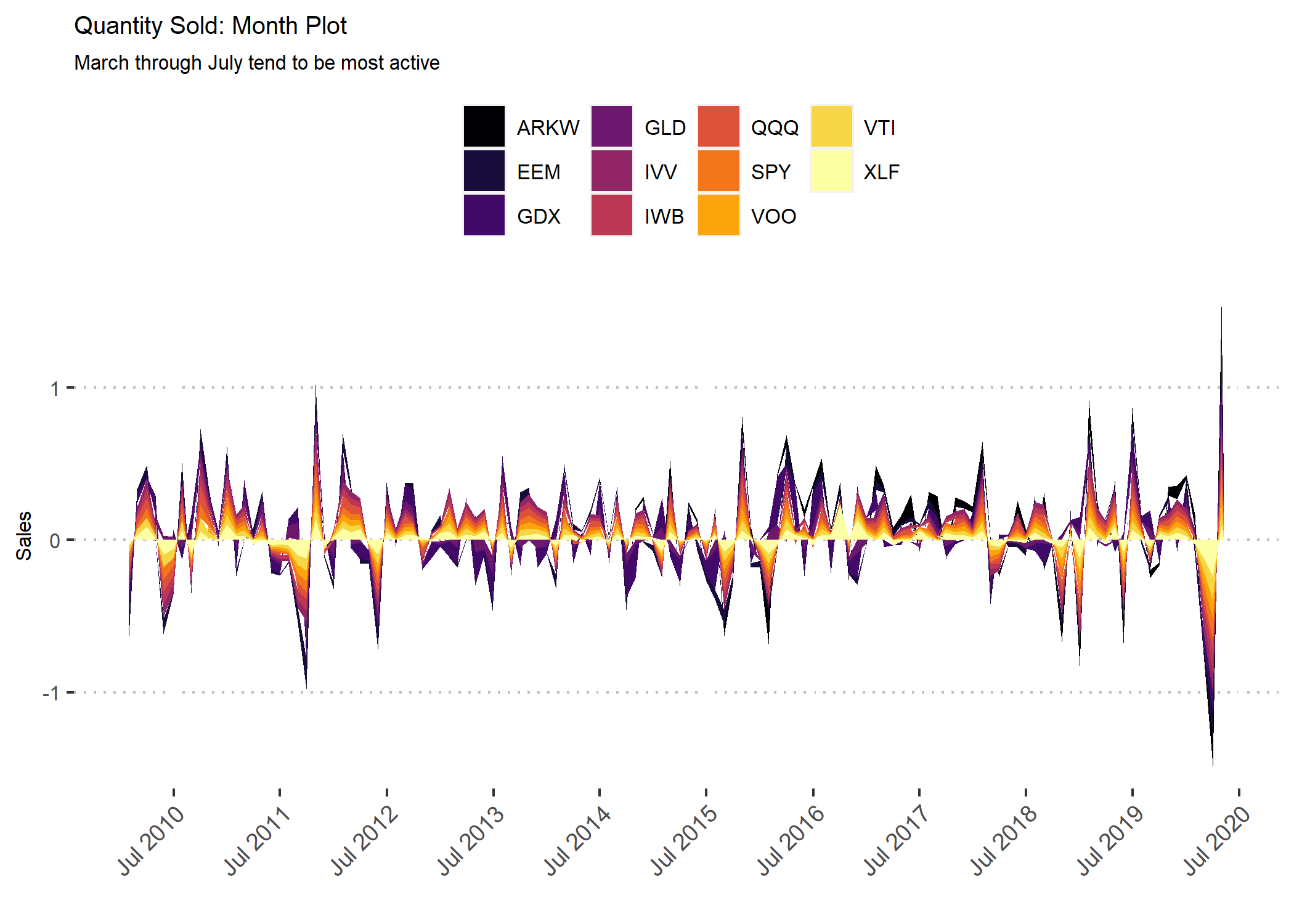
ETF_returns %>%
    ggplot(aes(x = date, y = monthly.returns, group = symbol)) +
    geom_area(aes(fill = symbol), position = "stack") +
    labs(title = "Quantity Sold: Month Plot", x = "", y = "Sales",
         subtitle = "March through July tend to be most active") +
    theme(
    legend.position="top",
    legend.direction="horizontal",
    legend.title = element_blank(),
    text=element_text(size=8,  family="Comic Sans MS"),
    axis.text.x=element_text(angle=45,hjust=1,size = 9),
    axis.text.y=element_text(size = 8),
    legend.text = element_text(size=8)
)+
    scale_x_date(breaks = date_breaks("12 month"),labels=date_format("%b %Y") ) +
   # theme_tq()+
  #scale_color_viridis()
 #scale_color_continuous_tableau()
   scale_fill_viridis(discrete = T,option="B")
#scale_color_viridis_d()