Cost-Sensitive Deep Learning For Imbalanced Dataset Classification

Introduction

Data with imbalanced target class occurs frequently in several domians such as credit card Fraud Detection ,insurance claim prediction, email spam detection, anomaly detection, outlier detection etc. Financial instituions loose millions of dollars every year to fraudulent financial transactions. It is important that these institutions are able to identify fraud to protect their customers and also reduce the financial losses that comes from fraudsters. The goal here is to predict fraudulent transactions to minimize loss to financial companies. For machine learning data with imbalanced target clases, the model evaluation metric is the AUC, the area under the ROC curve and the area under the precision-recall curve. The accuaracy metric is not useful in these situations since usually the proportion of the positive class in these situations is so low that even a naive classifier that predicts all transactions as fraudulent would result in a high accuracy. For example the dataset considered here, the proportion of negative examples is over 99% this a naive classifier can predict all transactions as legitimate and would be over 99% accuarate.

%config IPCompleter.greedy=True

import tensorflow as tf
from tensorflow import keras
import os
import tempfile
import matplotlib as mpl
import matplotlib.pyplot as plt
import numpy as np
import pandas as pd
import seaborn as sns
import sklearn
from sklearn.metrics import confusion_matrix
from sklearn.model_selection import train_test_split
from sklearn.preprocessing import StandardScaler
import datetime

mpl.rcParams['figure.figsize'] = (12, 10)
colors = plt.rcParams['axes.prop_cycle'].by_key()['color']

# svm with class weight on an imbalanced classification dataset
from numpy import mean
from sklearn.datasets import make_classification
from sklearn.model_selection import cross_val_score
from sklearn.model_selection import RepeatedStratifiedKFold
from sklearn.metrics import precision_recall_curve
from sklearn.metrics import roc_auc_score
from sklearn.svm import SVC
from imblearn.under_sampling import RandomUnderSampler # doctest: +NORMALIZE_WHITESPACE
from imblearn import under_sampling, over_sampling
from imblearn.over_sampling import SMOTE

# activate R magic to run R in google colab notebook
import rpy2
%load_ext rpy2.ipython

The rpy2.ipython extension is already loaded. To reload it, use:
  %reload_ext rpy2.ipython

%%R

install.packages("yardstick")
install.packages("glue")

Description of Data.

The datasets can be found on kaggle.The link to it is here. The datasets contains transactions made by credit cards in September 2013 by european cardholders. This dataset presents transactions that occurred in two days, where we have 492 frauds out of 284,807 transactions. The dataset is highly imbalanced, the positive class (frauds) account for 0.172% of all transactions.

It contains only numerical input variables which are the result of a PCA transformation. This was done to preserve the identity and privacy of the people whose transaction this data was gathered from. Features V1, V2, … V28 are the principal components obtained with PCA, the only features which have not been transformed with PCA are ‘Time’ and ‘Amount’. Feature ‘Time’ contains the seconds elapsed between each transaction and the first transaction in the dataset. The feature ‘Amount’ is the transaction Amount, this feature can be used for example-dependant cost-senstive learning. Feature ‘Class’ is the response variable and it takes value 1 in case of fraud and 0 otherwise.

df = pd.read_csv('/data/creditcard.csv')
df.head()

	Time	V1	V2	V3	V4	V5	V6	V7	V8	V9	...	V21	V22	V23	V24	V25	V26	V27	V28	Amount
0	0.0	-1.359807	-0.072781	2.536347	1.378155	-0.338321	0.462388	0.239599	0.098698	0.363787	...	-0.018307	0.277838	-0.110474	0.066928	0.128539	-0.189115	0.133558	-0.021053	149.62
1	0.0	1.191857	0.266151	0.166480	0.448154	0.060018	-0.082361	-0.078803	0.085102	-0.255425	...	-0.225775	-0.638672	0.101288	-0.339846	0.167170	0.125895	-0.008983	0.014724	2.69
2	1.0	-1.358354	-1.340163	1.773209	0.379780	-0.503198	1.800499	0.791461	0.247676	-1.514654	...	0.247998	0.771679	0.909412	-0.689281	-0.327642	-0.139097	-0.055353	-0.059752	378.66
3	1.0	-0.966272	-0.185226	1.792993	-0.863291	-0.010309	1.247203	0.237609	0.377436	-1.387024	...	-0.108300	0.005274	-0.190321	-1.175575	0.647376	-0.221929	0.062723	0.061458	123.50
4	2.0	-1.158233	0.877737	1.548718	0.403034	-0.407193	0.095921	0.592941	-0.270533	0.817739	...	-0.009431	0.798278	-0.137458	0.141267	-0.206010	0.502292	0.219422	0.215153	69.99

5 rows × 31 columns

df[['Time', 'V1', 'V2', 'V3', 'V4', 'V5', 'V26', 'V27', 'V28', 'Amount', 'Class']].describe().transpose()

	count	mean	std	min	25%	50%	75%	max
Time	284807.0	9.481386e+04	47488.145955	0.000000	54201.500000	84692.000000	139320.500000	172792.000000
V1	284807.0	3.919560e-15	1.958696	-56.407510	-0.920373	0.018109	1.315642	2.454930
V2	284807.0	5.688174e-16	1.651309	-72.715728	-0.598550	0.065486	0.803724	22.057729
V3	284807.0	-8.769071e-15	1.516255	-48.325589	-0.890365	0.179846	1.027196	9.382558
V4	284807.0	2.782312e-15	1.415869	-5.683171	-0.848640	-0.019847	0.743341	16.875344
V5	284807.0	-1.552563e-15	1.380247	-113.743307	-0.691597	-0.054336	0.611926	34.801666
V26	284807.0	1.699104e-15	0.482227	-2.604551	-0.326984	-0.052139	0.240952	3.517346
V27	284807.0	-3.660161e-16	0.403632	-22.565679	-0.070840	0.001342	0.091045	31.612198
V28	284807.0	-1.206049e-16	0.330083	-15.430084	-0.052960	0.011244	0.078280	33.847808
Amount	284807.0	8.834962e+01	250.120109	0.000000	5.600000	22.000000	77.165000	25691.160000
Class	284807.0	1.727486e-03	0.041527	0.000000	0.000000	0.000000	0.000000	1.000000

Examine the class label imbalance

The proportion of classs imbalance is evaluated below, the data is highly imbalanced.

df.Class.value_counts(normalize=True)*100

0    99.827251
1     0.172749
Name: Class, dtype: float64

neg, pos = df.Class.value_counts()
total = neg + pos
print('Examples:\n    Total: {}\n    Positive: {} ({:.2f}% of total)\n  '.format(
    total, pos, 100 * pos / total,100 * neg / total))

print('Total: {}\n    Negative: {} ({:.2f}% of total)\n  '.format(
    total, neg, 100 * neg / total))

Examples:
    Total: 284807
    Positive: 492 (0.17% of total)
  
Total: 284807
    Negative: 284315 (99.83% of total)

preprocesing Data

# The Time feature is not useful for our analysis and would be removed
#The pop() method returns the item present at the given index. This item is also removed from the list.
#df.pop('Time')
df = df.drop(['Time'],axis=1)

# The Amount feature
eps=0.00001 
df['Log Ammount'] = np.log(df.pop('Amount')+eps)

The dataset would be split into train, validation, and test sets. The train would be used in training, the validation set would be used toevaluate the model loss during training. The test setis an out-of-time set that is used to evaluate the performance of the model.Various metrics including Area Under the ROC-Curve, Area under the Precision-Recall curve, f-1 etc would be used to evaluate the model on the test data.

train_df, test_df = train_test_split(df, test_size=0.2)
train_df, val_df = train_test_split(train_df, test_size=0.2)
print('Traing dataset size:{}'.format(train_df.shape))
print('Test dataset size:{}'.format(test_df.shape))
print('Validation dataset size: {}'.format(val_df.shape))

Traing dataset size:(182276, 30)
Test dataset size:(56962, 30)
Validation dataset size: (45569, 30)

#obtain the target label by removing it   from the data splits above
train_labels = train_df.pop('Class')
val_labels =   val_df.pop('Class')
test_labels = np.array(test_df.pop('Class'))

from sklearn.preprocessing import MinMaxScaler



#Deep-learning models perform better with normalization, we choose the minmax normalization scheme here.
scaler = MinMaxScaler()
train_x = scaler.fit_transform(train_df)

val_x = scaler.transform(val_df)
test_x = scaler.transform(test_df)



print(' Training labels Shape:', train_labels.shape)
print('Validation labels shape:', val_labels.shape)
print('Test labels shape:', test_labels.shape)

print('Training features shape:', train_x.shape)
print('Validation features shape:', val_x.shape)
print('Test features shape:', test_x.shape)

Training labels shape: (182276,)
Validation labels shape: (45569,)
Test labels shape: (56962,)
Training features shape: (182276, 29)
Validation features shape: (45569, 29)
Test features shape: (56962, 29)

The target variable is a list, we convert to numpy arrays to prevent error that occured during training before this change.

train_labels = np.asarray(train_labels)
val_labels = np.asarray(val_labels)
test_labels =  np.asarray(test_labels)

Deep Learning

import tensorflow as tf
import tensorflow_hub as hub
import numpy as np
import matplotlib.pyplot as plt
try:
  # %tensorflow_version only exists in Colab.
  %tensorflow_version 2.x
except Exception:
  pass





batchsize=512
epoch=50

def plot_loss(history, label, n):
  # Use a log scale to show the wide range of values.
  plt.plot(history.epoch,  history.history['loss'],
               color=colors[n], label='Train '+label)
  plt.plot(history.epoch,  history.history['val_loss'],
          color=colors[n], label='Val '+label,
          linestyle="--")
  plt.xlabel('Epoch')
  plt.ylabel('Loss')
  
  plt.legend()

Check training history

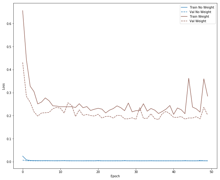
It is important to check the performance of the model on the validation set during training. This can give an idea as to whether some over-fitting is taking place, when the training loss keeps going down whereas the validation loss increase, this would would be an evidence of over-fitting. The evolution of the model accuracy in the case when we don’t have imbalanced data is also checked during the various epochs, it is expected that that training and validation accuracy would improve as number of epochs increases up to a point from which , overfitting can start to occur.

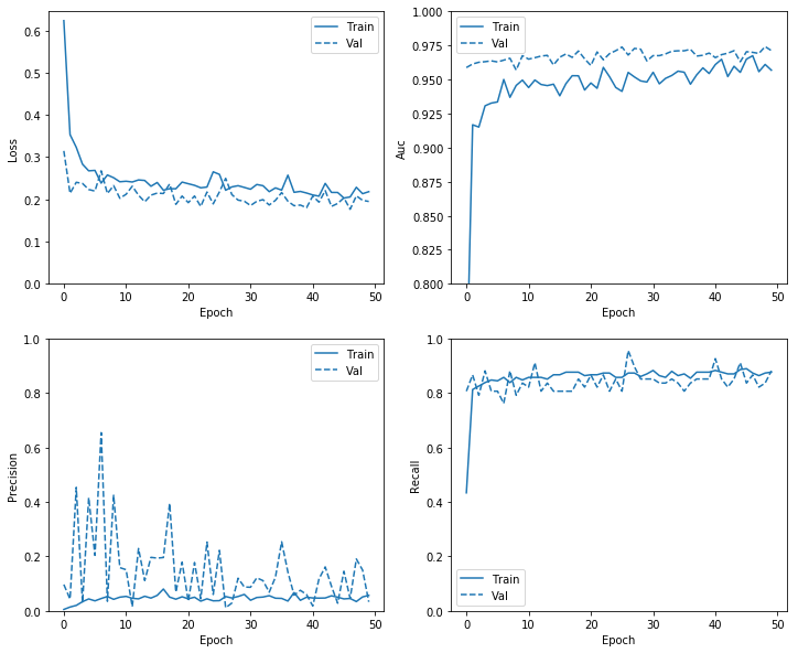
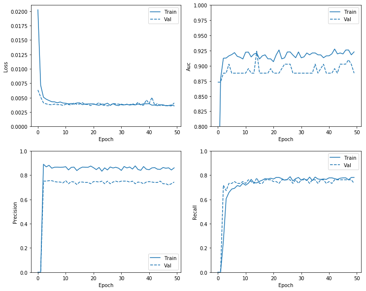
def plot_metrics(history):
  mpl.rcParams['figure.figsize'] = (12, 10)
  colors = plt.rcParams['axes.prop_cycle'].by_key()['color']  
  metrics =  ['loss', 'auc', 'precision', 'recall']
  for n, metric in enumerate(metrics):
    name = metric.replace("_"," ").capitalize()
    plt.subplot(2,2,n+1)
    plt.plot(history.epoch,  history.history[metric], color=colors[0], label='Train')
    plt.plot(history.epoch, history.history['val_'+metric],
             color=colors[0], linestyle="--", label='Val')
    plt.xlabel('Epoch')
    plt.ylabel(name)
    if metric == 'loss':
      plt.ylim([0, plt.ylim()[1]])
    elif metric == 'auc':
      plt.ylim([0.8,1])
    else:
      plt.ylim([0,1])

    plt.legend()

Search Over Weights

The deep learning model is set up below, it has 2 inner layers each with 128 nodes each. We would adopt empirical approach to find which weights/cost when placed on the target classes would minimize cost associated and improve the model performance. We can set up simple grid-search to explore this empirical process.

METRICS = [
      tf.keras.metrics.TruePositives(name='tp'),
      tf.keras.metrics.FalsePositives(name='fp'),
      tf.keras.metrics.TrueNegatives(name='tn'),
      tf.keras.metrics.FalseNegatives(name='fn'), 
      tf.keras.metrics.BinaryAccuracy(name='accuracy'),
      tf.keras.metrics.Precision(name='precision'),
      tf.keras.metrics.Recall(name='recall'),
      tf.keras.metrics.AUC(name='auc'),
]




def create_model(metrics = METRICS):
  
  model = tf.keras.Sequential([
      tf.keras.layers.Dense(
          128, activation='relu',
        input_shape=(train_df.shape[-1],), 
          kernel_initializer=tf.keras.initializers.glorot_normal()),
      tf.keras.layers.Dropout(0.5),
      tf.keras.layers.Dense(128, activation=tf.keras.activations.relu ,
                            kernel_initializer=tf.keras.initializers.glorot_normal()),  #'relu',
    tf.keras.layers.Dropout(0.5),
       tf.keras.layers.Dense(128, activation='relu'),
    tf.keras.layers.Dropout(0.5),
      tf.keras.layers.Dense(1, activation='sigmoid',
                            kernel_initializer= tf.keras.initializers.glorot_normal(), # tf.keras.initializers.RandomNormal,         #'random_uniform',
                            bias_initializer= tf.keras.initializers.RandomUniform(),  #minval=-0.05,maxval=1
                #bias_initializer= tf.keras.initializers.Constant(initial_bias)   #'zeros'
                #bias_initializer= tf.keras.initializers.Constant(value=0)
                            #bias_initializer= tf.keras.initializers.glorot_normal(seed=None)   #'zeros'
                #bias_initializer= tf.keras.initializers.VarianceScaling(scale=1.0, mode='fan_in', distribution='normal', seed=None)
                           ),
  ])

  model.compile(
      optimizer=tf.keras.optimizers.Adam(lr=1e-3),
      loss=tf.keras.losses.BinaryCrossentropy(),
      metrics=metrics)

  return model


model = create_model()
model.summary()

Model: "sequential"
_________________________________________________________________
Layer (type)                 Output Shape              Param #   
=================================================================
dense (Dense)                (None, 128)               3840      
_________________________________________________________________
dropout (Dropout)            (None, 128)               0         
_________________________________________________________________
dense_1 (Dense)              (None, 128)               16512     
_________________________________________________________________
dropout_1 (Dropout)          (None, 128)               0         
_________________________________________________________________
dense_2 (Dense)              (None, 128)               16512     
_________________________________________________________________
dropout_2 (Dropout)          (None, 128)               0         
_________________________________________________________________
dense_3 (Dense)              (None, 1)                 129       
=================================================================
Total params: 36,993
Trainable params: 36,993
Non-trainable params: 0
_________________________________________________________________

The cost-sensitive learning model is specified here as multi_weights model function below. We would experiment with different weights through a grid-search to determine which combination of weights provide the best performance.

# fit model
from sklearn.metrics import roc_auc_score



#for weight in  Target_weights:  
def multi_weights(weight):
    weight_model = create_model(metrics = METRICS)  
    #initial_bias_model = imbalanced_model(output_bias =initial_bias)
    weight_history = weight_model.fit(train_x, train_labels,
                    validation_data=(val_x,val_labels),
                    class_weight=weight,
                    batch_size=batchsize,    
                    epochs=epoch, 
                 
                    #callbacks=[early_stopping, mc,tensorboard],                  
                    verbose=0)
# evaluate model
    yhat = weight_model.predict(test_x)
    score = roc_auc_score(test_labels, yhat)
    #print('ROC AUC: %.3f'{} % score)
    #print('ROC AUC: %.5f : {}'.format(score))
    #tab=pd.DataFrame(Target_weights,score)
    
    return score
    

multi_weights({0:1, 1:20})

0.9772929746976037

# Scaling by total/2 helps keep the loss to a similar magnitude.
# The sum of the weights of all examples stays the same.
weight_for_0 = (1 / neg)*(total)/2.0 
weight_for_1 = (1 / pos)*(total)/2.0

class_weight = {0: weight_for_0, 1: weight_for_1}

print('Weight for class 0: {:.2f}'.format(weight_for_0))
print('Weight for class 1: {:.2f}'.format(weight_for_1))

Weight for class 0: 0.50
Weight for class 1: 289.44

The grid to search on is specified below, of course a larger grid could be considered if one has the luxury of larger computational power and time.

Target_weights=  [{0:0.05, 1:20},{0:1, 1:1},{0:0.5, 1:20},{0:1, 1:10},{0:1, 1:20},{0:1, 1:50},{0:1, 1:100},{0:1, 1:200},{0:1, 1:300},{0:1, 1:400},
                  {0:1, 1:500},{0:1, 1:1000},{0:0.5, 1:289.44},{0:1, 1:2000}]
my_scores= map(multi_weights, Target_weights)

my_scores=list(my_scores)

#Target_weights=  [{0:1, 1:100},{0:1, 1:200},{0:1, 1:500}]
t=pd.DataFrame(Target_weights,my_scores)
#t.columns=["Target_weights_0","Target_weights_1","my_scores"]
t=t.reset_index()
t.columns=["roc_auc_scores","Target_weights_0","Target_weights_1"]
print(t.shape)

#Target_weights
#Target_weights[0:2][0]
t.style.set_properties(**{'background-color': 'pink',
                            'color': 'black',
                            'border-color': 'white'})



t.style.clear()
import seaborn as sns

cm = sns.light_palette("green", as_cmap=True)
s= t.style.background_gradient(cmap=cm)
s

(14, 3)

	roc_auc_scores	Target_weights_0	Target_weights_1
0	0.981511	0.05	20
1	0.977042	1	1
2	0.975231	0.5	20
3	0.97277	1	10
4	0.975759	1	20
5	0.974144	1	50
6	0.978512	1	100
7	0.975634	1	200
8	0.976383	1	300
9	0.978398	1	400
10	0.976865	1	500
11	0.981105	1	1000
12	0.982826	0.5	289.44
13	0.980766	1	2000

The no_weights model is the reference model that the cost-sensitive learning would be compared to, it is specified below.No weights implies the cost assigned to both minority and majority classes is the same taken to be 1.

def no_weights(weight):
    no_weight_model = create_model()
    #initial_bias_model = imbalanced_model(output_bias =initial_bias)
    no_weight_history = no_weight_model.fit(train_x, train_labels,
                    validation_data=(val_x,val_labels),
                    class_weight=weight,
                    batch_size=batchsize,    
                    epochs=epoch, 
                    #callbacks=[early_stopping, mc,tensorboard],                         
                    verbose=0)
# evaluate model
    yhat = no_weight_model.predict(test_x)
    score = roc_auc_score(test_labels, yhat)
    #print('ROC AUC: %.3f'{} % score)
    #print('ROC AUC: %.5f : {}'.format(score))
    #tab=pd.DataFrame(Target_weights,score)
    
    return score   

The weight that generates the maximum AUC of 0.982826 is {0:0.5, 1:289.44}. The weights {0:0.05, 1:20} comes very close with AUC of 0.981511.

colors=['#FFFF00','#FFFF00','#58FAF4','#F6CECE','#000000','#AC58FA']


weight_model = create_model()
weight_history = weight_model.fit(train_x, train_labels,
                    validation_data=(val_x,val_labels),
                    class_weight={0:0.5, 1:289.44},
                    batch_size=batchsize,    
                    epochs=epoch, 
                    # callbacks=[early_stopping, mc,tensorboard],              
                    verbose=0)

no_weight_model = create_model()
no_weight_history = no_weight_model.fit(train_x, train_labels,
                    validation_data=(val_x,val_labels),
                    class_weight={0:1, 1:1},
                    batch_size=batchsize,    
                    epochs=epoch, 
                    #callbacks=[early_stopping, mc,tensorboard],              
                    verbose=0)

#weight_history.history["recall"]

%matplotlib inline

def plot_loss(history, label, n):
  # Use a log scale to show the wide range of values.
  plt.plot(history.epoch,  history.history['loss'],
               color=colors[n], label='Train '+label)
  plt.plot(history.epoch,  history.history['val_loss'],
          color=colors[n], label='Val '+label,
          linestyle="--")
  plt.xlabel('Epoch')
  plt.ylabel('Loss')
  
  plt.legend()


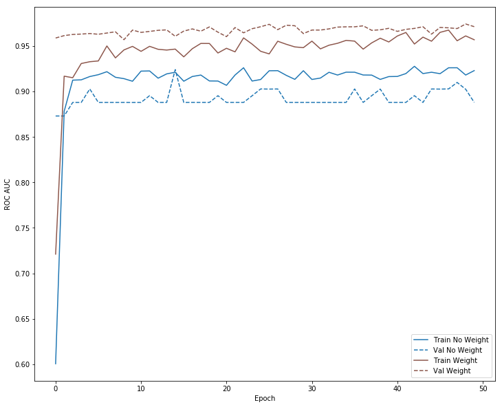
def plot_auc(history, label, n):
  # Use a log scale to show the wide range of values.
  plt.plot(history.epoch,  history.history['auc'],
               color=colors[n], label='Train '+label)
  plt.plot(history.epoch,  history.history['val_auc'],
          color=colors[n], label='Val '+label,
          linestyle="--")
  plt.xlabel('Epoch')
  plt.ylabel('ROC AUC')
  
  plt.legend()


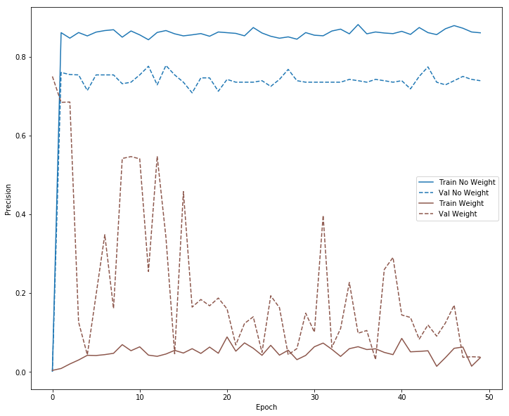
def plot_precision(history, label, n):
  # Use a log scale to show the wide range of values.
  plt.plot(history.epoch,  history.history['precision'],
               color=colors[n], label='Train '+label)
  plt.plot(history.epoch,  history.history['val_precision'],
          color=colors[n], label='Val '+label,
          linestyle="--")
  plt.xlabel('Epoch')
  plt.ylabel('Precision')
  
  plt.legend()



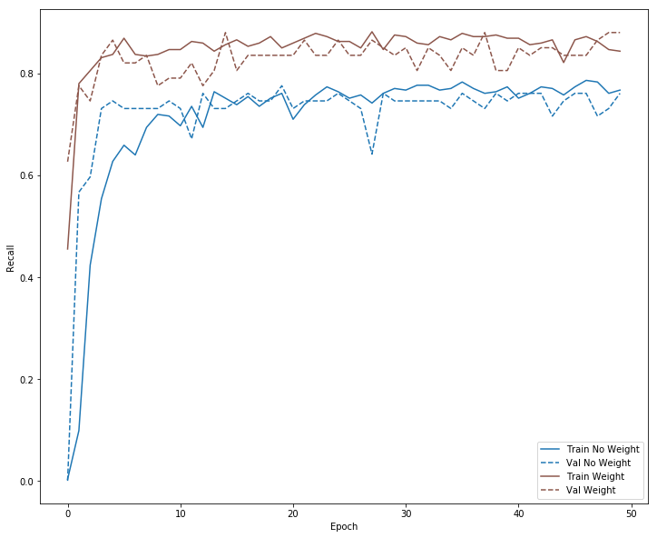
def plot_recall(history, label, n):
  # Use a log scale to show the wide range of values.
  plt.plot(history.epoch,  history.history['recall'],
               color=colors[n], label='Train '+label)
  plt.plot(history.epoch,  history.history['val_recall'],
          color=colors[n], label='Val '+label,
          linestyle="--")
  plt.xlabel('Epoch')
  plt.ylabel('Recall')
  
  plt.legend()

mpl.rcParams['figure.figsize'] = (12, 10)
colors = plt.rcParams['axes.prop_cycle'].by_key()['color']
plot_loss(no_weight_history, "No Weight", 0)
plot_loss(weight_history, "Weight", 5)
plt.savefig('loss.png')

png

mpl.rcParams['figure.figsize'] = (12, 10)
colors = plt.rcParams['axes.prop_cycle'].by_key()['color']
plot_auc(no_weight_history, "No Weight", 0)
plot_auc(weight_history, "Weight", 5)
plt.savefig('rocauc.png')

png

mpl.rcParams['figure.figsize'] = (12, 10)
colors = plt.rcParams['axes.prop_cycle'].by_key()['color']
plot_precision(no_weight_history, "No Weight", 0)
plot_precision(weight_history, "Weight", 5)
plt.savefig('precision.png')

png

mpl.rcParams['figure.figsize'] = (12, 10)
colors = plt.rcParams['axes.prop_cycle'].by_key()['color']
plot_recall(no_weight_history, "No Weight", 0)
plot_recall(weight_history, "Weight", 5)
plt.savefig('recall.png')

png

plot_metrics(weight_history )

png

plot_metrics(no_weight_history )

png

from __future__ import absolute_import, division, print_function, unicode_literals

import os

#!pip install --upgrade tensorflow

import tensorflow as tf
from tensorflow import keras

print(tf.version.VERSION)
#from terminal python -c 'import tensorflow as tf; print(tf.__version__)'
#pip install --user <package_name>
#Example,

#pip install --user tensorflow

2.0.0

The trained save modmodel can be saved to file and loaded for later use.

# Save the model
no_weight_model.save('no_weight_model.h5')
weight_model.save('weight_model.h5')

# Recreate the exact same model purely from the file
#new_model = tf.keras.models.load_model('path_to_my_model.h5')

The model weights values can be saved to file as below. The weights values can be retrieved as a list of Numpy arrays via get_weights(), and set the state of the model via set_weights:

weights = weight_model.get_weights()  # Retrieves the state of the model.
weight_model.set_weights(weights)  # Sets the state of the model.

no_weights = no_weight_model.get_weights()  # Retrieves the state of the model.
no_weight_model.set_weights(no_weights)  # Sets the state of the model.

test_predictions_no_weight = no_weight_model.predict(test_x, batch_size=batchsize)
test_predictions_weight =    weight_model.predict(test_x, batch_size=batchsize)
train_predictions_no_weight  = no_weight_model.predict(train_x, batch_size=batchsize)
train_predictions_weight = weight_model.predict(train_x, batch_size=batchsize)

from sklearn.metrics import classification_report
p=0.5

def PlotConfusionMatrix(y_test,pred,y_test_legit,y_test_fraud,label):

    cfn_matrix = confusion_matrix(y_test,pred)
    cfn_norm_matrix = np.array([[1.0 / y_test_legit,1.0/y_test_legit],[1.0/y_test_fraud,1.0/y_test_fraud]])
    norm_cfn_matrix = cfn_matrix * cfn_norm_matrix

    #colsum=cfn_matrix.sum(axis=0)
    #norm_cfn_matrix = cfn_matrix / np.vstack((colsum, colsum)).T

    fig = plt.figure(figsize=(15,5))
    ax = fig.add_subplot(1,2,1)
    sns.heatmap(cfn_matrix,cmap='magma',linewidths=0.5,annot=True,ax=ax)
    #tick_marks = np.arange(len(y_test))
    #plt.xticks(tick_marks, np.unique(y_test), rotation=45)
    plt.title('Confusion Matrix')
    plt.ylabel('Real Classes')
    plt.xlabel('Predicted Classes')
    plt.savefig('cm_' +label +  '.png')
        
    ax = fig.add_subplot(1,2,2)
    sns.heatmap(norm_cfn_matrix,cmap=plt.cm.Blues,linewidths=0.5,annot=True,ax=ax)

    plt.title('Normalized Confusion Matrix')
    plt.ylabel('Real Classes')
    plt.xlabel('Predicted Classes')
    plt.savefig('cm_norm' +label +  '.png')
    plt.show()
    
    print('---Classification Report---')
    print(classification_report(y_test,pred))
    
    # Let's store our y_test legit and fraud counts for normalization purposes later on
#y_test_legit = y_test.value_counts()[0]
#y_test_fraud = y_test.value_counts()[1]
#y_test_legit = np.count_nonzero(y_test == -1)
#y_test_fraud = np.count_nonzero(y_test == 1)


y_test_legit,y_test_fraud = np.bincount(test_labels)
y_pred= np.where(test_predictions_weight<p,0,1 )


PlotConfusionMatrix(test_labels,y_pred,y_test_legit,y_test_fraud,label='weight')

#plt.savefig('cm_weights.png')

png

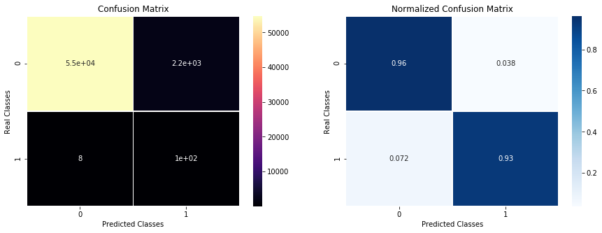
---Classification Report---
              precision    recall  f1-score   support

           0       1.00      0.96      0.98     56851
           1       0.05      0.93      0.09       111

   micro avg       0.96      0.96      0.96     56962
   macro avg       0.52      0.95      0.53     56962
weighted avg       1.00      0.96      0.98     56962

y_test_legit,y_test_fraud = np.bincount(test_labels)
y_pred= np.where(test_predictions_no_weight<0.5,0,1 )
PlotConfusionMatrix(test_labels,y_pred,y_test_legit,y_test_fraud,label="noweight")

plt.savefig('cm_noweights.png')

png

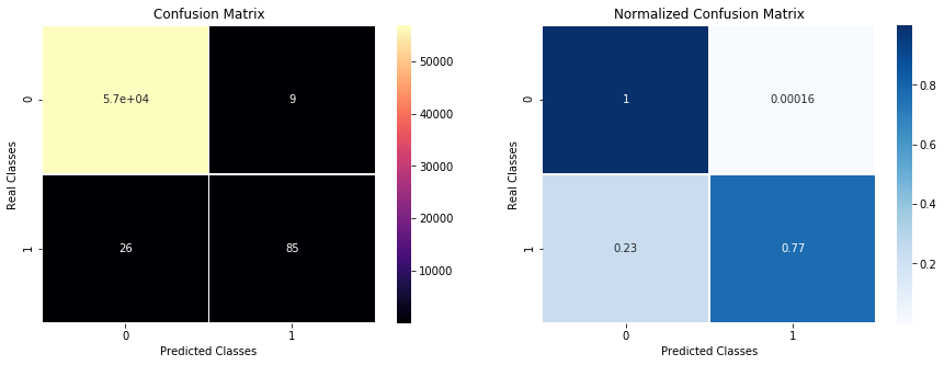
---Classification Report---
              precision    recall  f1-score   support

           0       1.00      1.00      1.00     56851
           1       0.90      0.77      0.83       111

   micro avg       1.00      1.00      1.00     56962
   macro avg       0.95      0.88      0.91     56962
weighted avg       1.00      1.00      1.00     56962

<Figure size 864x720 with 0 Axes>

#help(confusion_matrix)

Placing weights on the target variable to increase the true positive rate also comes with a cost , the precision rate decreases because the false positive rates increases. Increasing the true positive rate at the expense of false positive rate should be a decision that can be made depending on the particular application. In the case of fraud detection, high false positive means high number of legitimate transactions that were incorrectly flagged as fraudulent.This can create inconvenience and dissatisfaction among customers. Higher false negative rate is however more costly since fraudulent transactions would be declared as legitimate.

from sklearn.metrics import precision_score
from sklearn.metrics import recall_score
from sklearn.metrics import precision_recall_fscore_support
from numpy import trapz
from scipy.integrate import simps
from sklearn.metrics import f1_score

def Evaluate(labels, predictions, p=0.5):
    CM= confusion_matrix(labels, predictions > p)
    TN = CM[0][0]
    FN = CM[1][0]
    TP = CM[1][1]
    FP = CM[0][1]
    print('Legitimate Transactions Detected (True Negatives): {}'.format(TN))
    print('Fraudulent Transactions Missed (False Negatives):  {}'.format(FN))
    print('Fraudulent Transactions Detected (True Positives): {}'.format(TP))
    print('Legitimate Transactions Incorrectly Detected (False Positives):{}'.format(FP))
    print('Total Fraudulent Transactions: ', np.sum(CM[1]))
    auc = roc_auc_score(labels, predictions)
    prec=precision_score(labels, predictions>p)
    rec=recall_score(labels, predictions>p)
     # calculate F1 score
    f1 = f1_score(labels, predictions>p)
    print('auc :{}'.format(auc))
    print('precision :{}'.format(prec))
    print('recall :{}'.format(rec))
    print('f1 :{}'.format(f1))
    # Compute Precision-Recall and plot curve
    precision, recall, thresholds = precision_recall_curve(labels, predictions>p)
    #use the trapezoidal rule to calculate the area under the precion-recall curve
    area =  trapz(recall, precision)
    #area =  simps(recall, precision)
    print("Area Under PR Curve(AP): %0.4f" % area)   #should be same as AP?    

#yhat = weight_model.predict(test_x)
yhat = test_predictions_no_weight 
Evaluate(labels=test_labels, predictions=yhat, p=0.5)

Legitimate Transactions Detected (True Negatives): 56842
Fraudulent Transactions Missed (False Negatives):  26
Fraudulent Transactions Detected (True Positives): 85
Legitimate Transactions Incorrectly Detected (False Positives):9
Total Fraudulent Transactions:  111
auc :0.9686300256035177
precision :0.9042553191489362
recall :0.7657657657657657
f1 :0.8292682926829268
Area Under PR Curve(AP): 0.8333

#yhat = weight_model.predict(test_x)
yhat = test_predictions_weight

Evaluate(labels=test_labels, predictions=yhat, p=0.5)

Legitimate Transactions Detected (True Negatives): 54700
Fraudulent Transactions Missed (False Negatives):  8
Fraudulent Transactions Detected (True Positives): 103
Legitimate Transactions Incorrectly Detected (False Positives):2151
Total Fraudulent Transactions:  111
auc :0.9807726408577757
precision :0.04569653948535936
recall :0.9279279279279279
f1 :0.08710359408033826
Area Under PR Curve(AP): 0.4849

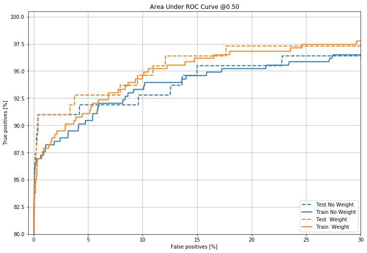
Plot the AUC ROC

from sklearn.metrics import roc_curve

def plot_roc(name, labels, predictions, p=0.5, **kwargs):
  fp, tp, _ = sklearn.metrics.roc_curve(labels, predictions)

  plt.plot(100*fp, 100*tp, label=name, linewidth=2, **kwargs)
  plt.xlabel('False positives [%]')
  plt.ylabel('True positives [%]')
  plt.xlim([-0.5,30])
  plt.title('Area Under ROC Curve @{:.2f}'.format(p))
  plt.ylim([80,100.5])
  plt.grid(True)
  ax = plt.gca()
  ax.set_aspect('equal')



plot_roc("Test No Weight", test_labels, test_predictions_no_weight, color=colors[0],linestyle='--')
plot_roc("Train No Weight", train_labels, train_predictions_no_weight, color=colors[0])

plot_roc("Test  Weight", test_labels, test_predictions_weight, color=colors[1], linestyle='--')
plot_roc("Train  Weight", train_labels, train_predictions_weight, color=colors[1])


plt.legend(loc='lower right')

plt.savefig('t_rocauc.png')

png

Plot the Area Under Precision Recall Curve

from sklearn.metrics import precision_recall_curve

def plot_auc_pr(name, labels, predictions,n=0.5, **kwargs):
  p, r, _ = sklearn.metrics.precision_recall_curve(labels, predictions)

  plt.plot(100*r, 100*p, label=name, linewidth=2, **kwargs)
  plt.xlabel('Recall [%]')
  plt.ylabel('Precision [%]')
  plt.xlim([-0.5,100])
  plt.title('Area Under Precision-Recall Curve @{:.2f}'.format(n))
  #plt.title('Area Under Precision-Recall Curve: {}' .format(p))
  plt.ylim([0,100.5])
  plt.grid(True)
  ax = plt.gca()
  ax.set_aspect('equal')


#plot_auc_pr("Train Baseline", test_labels,test_predictions_no_weight, color=colors[0])
#plot_auc_pr("Test Baseline", test_labels, test_predictions_weight, color=colors[1], linestyle='--')


plot_auc_pr("Test No Weight", test_labels, test_predictions_no_weight, color=colors[0],linestyle='--')
plot_auc_pr("Train No Weight", train_labels, train_predictions_no_weight, color=colors[0])

plot_auc_pr("Test  Weight", test_labels, test_predictions_weight, color=colors[1], linestyle='--')
plot_auc_pr("Train  Weight", train_labels, train_predictions_weight, color=colors[1])

plt.legend(loc='upper right')
plt.savefig('all_aupr.png')

png

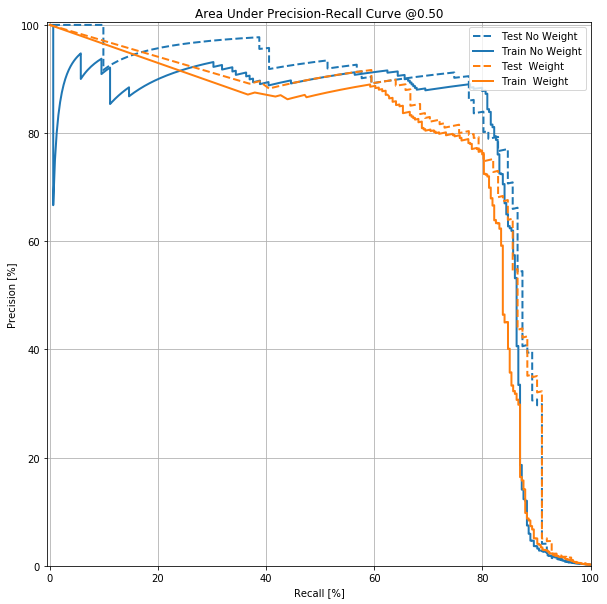
Sampling Based Approaches

Under-Sampling

In Under-sampling, the samples majority class is randomly eliminated until there is a balance between the distribution both target classes. This could lead to loss of useful information.

from collections import Counter
from sklearn.datasets import make_classification
from imblearn.under_sampling import RandomUnderSampler # doctest: +NORMALIZE_WHITESPACE


rus = RandomUnderSampler(random_state=42)
X_rus, y_rus = rus.fit_resample(train_x,  train_labels)
print('Resampled dataset shape %s' % Counter(y_rus))



undersampling_model = create_model()
undersampling_history = undersampling_model.fit(X_rus, y_rus,
                    validation_data=(val_x,val_labels),
                    class_weight={0:1, 1:1},
                    batch_size=batchsize,    
                    epochs=epoch, 
                    #callbacks=[early_stopping, mc,tensorboard],              
                    verbose=0)

# evaluate model
yhat = undersampling_model.predict(test_x)
Evaluate(labels=test_labels, predictions=yhat, p=0.5)

Resampled dataset shape Counter({0: 314, 1: 314})
Legitimate Transactions Detected (True Negatives): 56132
Fraudulent Transactions Missed (False Negatives):  11
Fraudulent Transactions Detected (True Positives): 100
Legitimate Transactions Incorrectly Detected (False Positives):719
Total Fraudulent Transactions:  111
auc :0.9788451271626589
precision :0.1221001221001221
recall :0.9009009009009009
f1 :0.21505376344086022
Area Under PR Curve(AP): 0.5096

SMOTE

This method involves over-sampling the minority class by creating synthetic minority class examples.The minority class is over-sampled by creating “synthetic” examples rather than by over-sampling with replacement. All minority examples are kept, and synthetic examples are created by sampling from the k-nearest neighbors of these minority examples.

from collections import Counter
from sklearn.datasets import make_classification
from imblearn.over_sampling import SMOTE # doctest: +NORMALIZE_WHITESPACE

print('Original dataset shape %s' % Counter(train_labels))

sm = SMOTE(random_state=42)

X_smote, y_smote = sm.fit_resample(train_x,  train_labels)

smote_model = create_model()
smote_history = smote_model.fit(X_smote, y_smote,
                    validation_data=(val_x,val_labels),
                    class_weight={0:1, 1:1},
                    batch_size=batchsize,    
                    epochs=epoch, 
                    #callbacks=[early_stopping, mc,tensorboard],              
                    verbose=0)

# evaluate model
yhat = smote_model.predict(test_x)
Evaluate(labels=test_labels, predictions=yhat, p=0.5)

Original dataset shape Counter({0: 181962, 1: 314})
Legitimate Transactions Detected (True Negatives): 55708
Fraudulent Transactions Missed (False Negatives):  7
Fraudulent Transactions Detected (True Positives): 104
Legitimate Transactions Incorrectly Detected (False Positives):1143
Total Fraudulent Transactions:  111
auc :0.98526565650275
precision :0.08340016038492382
recall :0.9369369369369369
f1 :0.15316642120765828
Area Under PR Curve(AP): 0.5083

Over-Sampling

Over-sampling works by replicating or creating additional copies of the minority class to balance the distribution of the target class.This approach is known to potentially cause over-fitting and computationally expensive.

from collections import Counter
from sklearn.datasets import make_classification
#from imblearn.under_sampling import RandomOverSampler # doctest: +NORMALIZE_WHITESPACE
from imblearn import under_sampling, over_sampling
from imblearn.over_sampling import RandomOverSampler

rus = RandomOverSampler(random_state=42)
X_rus, y_rus = rus.fit_resample(train_x,  train_labels)
print('Resampled dataset shape %s' % Counter(y_rus))


oversampling_model = create_model()
oversampling_history = oversampling_model.fit(X_rus, y_rus,
                    validation_data=(val_x,val_labels),
                    class_weight={0:1, 1:1},
                    batch_size=batchsize,    
                    epochs=epoch, 
                    #callbacks=[early_stopping, mc,tensorboard],              
                    verbose=0)

# evaluate model
yhat = oversampling_model.predict(test_x)
Evaluate(labels=test_labels, predictions=yhat, p=0.5)

Resampled dataset shape Counter({0: 181962, 1: 181962})
Legitimate Transactions Detected (True Negatives): 54797
Fraudulent Transactions Missed (False Negatives):  6
Fraudulent Transactions Detected (True Positives): 105
Legitimate Transactions Incorrectly Detected (False Positives):2054
Total Fraudulent Transactions:  111
auc :0.9823669776265157
precision :0.04863362667901806
recall :0.9459459459459459
f1 :0.09251101321585903
Area Under PR Curve(AP): 0.4954

test_predictions_no_weight = no_weight_model.predict(test_x, batch_size=batchsize)
test_predictions_weight =    weight_model.predict(test_x, batch_size=batchsize)
test_predictions_oversampling= oversampling_model.predict(test_x, batch_size=batchsize)
test_predictions_smote =    smote_model.predict(test_x, batch_size=batchsize)
test_predictions_undersampling=    undersampling_model.predict(test_x, batch_size=batchsize)

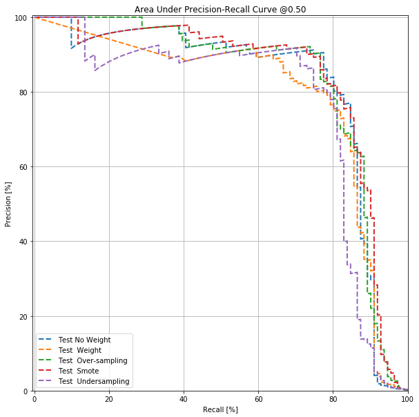
plot_auc_pr("Test No Weight", test_labels, test_predictions_no_weight, color=colors[0],linestyle='--')
plot_auc_pr("Test  Weight", test_labels, test_predictions_weight, color=colors[1],linestyle='--')
plot_auc_pr("Test  Over-sampling", test_labels, test_predictions_oversampling, color=colors[2],linestyle='--')
plot_auc_pr("Test  Smote", test_labels, test_predictions_smote, color=colors[3],linestyle='--')
plot_auc_pr("Test  Undersampling", test_labels, test_predictions_undersampling, color=colors[4],linestyle='--')
plt.legend(loc='lower left')
plt.savefig('1_aupr.png')

png

plot_roc("Test No Weight", test_labels, test_predictions_no_weight, color=colors[0],linestyle='--')
plot_roc("Test  Weight", test_labels, test_predictions_weight, color=colors[1],linestyle='--')
plot_roc("Test  Over-sampling", test_labels, test_predictions_oversampling, color=colors[2],linestyle='--')
plot_roc("Test  Smote", test_labels, test_predictions_smote, color=colors[3],linestyle='--')
plot_roc("Test  Undersampling", test_labels, test_predictions_undersampling, color=colors[4],linestyle='--')
plt.legend(loc='upper left')
plt.savefig('1_auc.png')

png

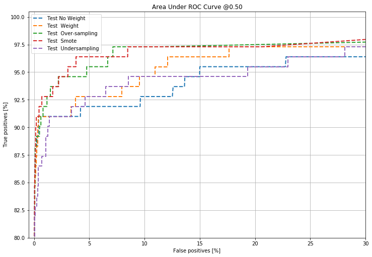
Fom this analysis, it appears that cost-sensitive deep learning models outperform other approaches to dealing with class imbalance namely SMOTE, oversampling, undersampling especially if the chosen evaluation metric is the AUC. These proposed methods for addressing class imbalance pays a penalty by sacrificing lower precision values for a higher recall values. The AUC has been criticized for leading to misleading conclusions in evaluating binary models although it is still the most popular evaluation metric for binary classifications model. The area under the precision-recall curve has been suggested an alternative to the AUC in imbalanced classification modeling.