Transfer Learning and Fine-Tuning with TensorFlow

Transfer learning involves taking layers/learned features from a model trained on a larger dataset and using those features to initialize training on another similar task. Training deep learning models especially for computer vision requires massive data to perform well. Transfer learning allows models to be trained on smaller dataset by taking advantage of features already learned by a bigger model to initialize training. In Transfer learning, the layers before the last or some number of layers is usually frozen and last layer modified depending on the number of target classes required in a particular task. Training occurs only on the last or the layers which is not frozen.

One popular model for transfer learning is the VGG-16 model trained on the ImageNet dataset. Imagenet is a dataset of over 15 million labeled high-resolution images belonging to roughly 22,000 categories. Fine-tuning which is usually performed to improve the transfer learning performance involves un-freezing all the layers and training on them new dataset with a very small learning rate.

The development version of tensorflow makes a lot of the preprocessing steps in image classification very straight-forward. It can be installed as below:

!pip install tf-nightly --quiet

[K     |████████████████████████████████| 323.8MB 51kB/s 
[K     |████████████████████████████████| 6.7MB 60.6MB/s 
[K     |████████████████████████████████| 460kB 54.1MB/s 
[?25h

import numpy as np
import tensorflow as tf
from tensorflow import keras
#from tensorflow.keras.preprocessing.image import image_dataset_from_directory
from keras import  layers
import matplotlib.pyplot as plt
import matplotlib as mpl
import os
mpl.rcParams['figure.figsize'] = (12, 10)
colors = plt.rcParams['axes.prop_cycle'].by_key()['color']
%autosave 5
print(tf.__version__)

Using TensorFlow backend.

Autosaving every 5 seconds
2.4.0-dev20200802

The Chest X-Ray Images (Pneumonia) dataset can be downloaded from kaggle from this link.

from google.colab import drive
import glob
drive.mount('/content/drive', force_remount=True)

Mounted at /content/drive

checkpointpath="/content/drive/My Drive/Colab Notebooks/ComputerVision/"

!unzip -q '/content/drive/My Drive/Data/chest_xray.zip'

!ls chest_xray/chest_xray/train/*/*  -U | head -4

chest_xray/chest_xray/train/NORMAL/IM-0115-0001.jpeg
chest_xray/chest_xray/train/NORMAL/IM-0117-0001.jpeg
chest_xray/chest_xray/train/NORMAL/IM-0119-0001.jpeg
chest_xray/chest_xray/train/NORMAL/IM-0122-0001.jpeg

Counting Files in the Current Directory

The number of training images is about 5216

!ls chest_xray/chest_xray/train/*/*.jpeg | wc -l

The number of pneumonia images is found below. The data is imbalanced as there is 3875 pneumonia images compared with 1341 normal or healthy images.

!ls chest_xray/chest_xray/train/PNEUMONIA/*.jpeg | wc -l

The number of images which is normal found below

!ls chest_xray/chest_xray/train/NORMAL/*.jpeg | wc -l

There are only 19 validation images. This is too few for any meaningful analysis, therefore the training dataset will be split into training and validataion for the anlysis below.

!ls chest_xray/chest_xray/val/*/ | wc -l

!ls chest_xray/chest_xray/val/*/

chest_xray/chest_xray/val/NORMAL/:
NORMAL2-IM-1427-0001.jpeg  NORMAL2-IM-1436-0001.jpeg  NORMAL2-IM-1440-0001.jpeg
NORMAL2-IM-1430-0001.jpeg  NORMAL2-IM-1437-0001.jpeg  NORMAL2-IM-1442-0001.jpeg
NORMAL2-IM-1431-0001.jpeg  NORMAL2-IM-1438-0001.jpeg

chest_xray/chest_xray/val/PNEUMONIA/:
person1946_bacteria_4874.jpeg  person1950_bacteria_4881.jpeg
person1946_bacteria_4875.jpeg  person1951_bacteria_4882.jpeg
person1947_bacteria_4876.jpeg  person1952_bacteria_4883.jpeg
person1949_bacteria_4880.jpeg  person1954_bacteria_4886.jpeg

!ls chest_xray/chest_xray/test/*/ -U | head -4

chest_xray/chest_xray/test/NORMAL/:
IM-0069-0001.jpeg
NORMAL2-IM-0201-0001.jpeg
NORMAL2-IM-0112-0001.jpeg

The test set count is about 627 images

!ls chest_xray/chest_xray/test/*/ | wc -l

!ls /content

chest_xray  drive  sample_data

!ls /content/*

/content/chest_xray:
chest_xray  __MACOSX  test  train  val

/content/drive:
'My Drive'

/content/sample_data:
anscombe.json		      mnist_test.csv
california_housing_test.csv   mnist_train_small.csv
california_housing_train.csv  README.md

!ls 'chest_xray/chest_xray/train'

NORMAL	PNEUMONIA

!ls 'chest_xray/chest_xray/train'

NORMAL	PNEUMONIA

Generate a Dataset

image_size = (180, 180)
batch_size = 32
input_shape=image_size + (3,)
# number of output classes
num_classes = 1

class_names  =['NORMAL','PNEUMONIA']

#train_ds = tf.keras.preprocessing.image_dataset_from_directory(
#    'chest_xray/chest_xray/train', seed=1337,
#    image_size=image_size, batch_size=batch_size)
#val_ds = tf.keras.preprocessing.image_dataset_from_directory(
#    'chest_xray/chest_xray/val', seed=1337,
#    image_size=image_size, batch_size=batch_size)

#print(input_shape)


train_ds = tf.keras.preprocessing.image_dataset_from_directory(
    'chest_xray/chest_xray/train', 
    validation_split=0.2, subset='training',
     seed=1337,
    image_size=image_size, batch_size=batch_size,
    labels= "inferred",
    class_names= class_names)
val_ds = tf.keras.preprocessing.image_dataset_from_directory(
    'chest_xray/chest_xray/train', validation_split=0.2, subset='validation', seed=1337,
    image_size=image_size, 
     labels= "inferred",
     class_names= class_names,
    batch_size=batch_size)

print(input_shape)

Found 5216 files belonging to 2 classes.
Using 4173 files for training.
Found 5216 files belonging to 2 classes.
Using 1043 files for validation.
(180, 180, 3)

#print(next(iter(val_ds.take(1))))

test_ds = tf.keras.preprocessing.image_dataset_from_directory(
    'chest_xray/chest_xray/test', seed=1337,
    image_size=image_size, 
     labels= "inferred",
     class_names= class_names,
     batch_size=batch_size)

Found 624 files belonging to 2 classes.

class_names = train_ds.class_names
print(class_names)

['NORMAL', 'PNEUMONIA']

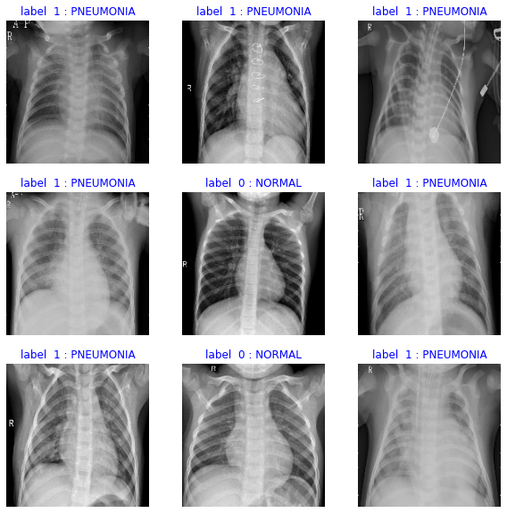
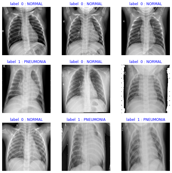
Some of the images can be randomly selected and visualized as done below.

import matplotlib.pyplot as plt

plt.figure(figsize=(10, 10))
#for images, labels in train_ds.take(1):
for i, (images, labels) in enumerate(train_ds.take(9)):
#  for i in range(9):
    ax = plt.subplot(3, 3, i + 1)
    plt.imshow(images[i].numpy().astype("uint8"))
    #plt.title(class_names[labels[i]])
    plt.title("label  {n} : {s}".format(n=labels[i].numpy(), s=class_names[labels[i]]),color='b')  
    #plt.title("Label %s : %s" % (labels[i].numpy(), class_names[labels[i]]))
    plt.axis("off")
    plt.savefig("/content/drive/My Drive/Colab Notebooks/ComputerVision/image1.png")

png

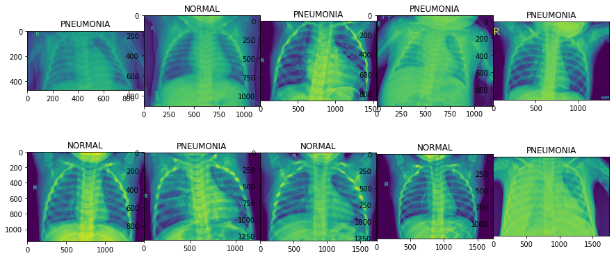
Equivalently, we also randomly select some images from the training data to visualize.

import itertools 
train_filenames = glob.glob('chest_xray/chest_xray/train/*/*')
test_filenames = glob.glob('chest_xray/chest_xray/test/*/*')
#filenames[0:5]
rand_image = [train_filenames[i] for i in np.random.randint(len(train_filenames), size=10)]
#rand_image = list(itertools.compress(filenames, np.random.randint(len(filenames), size=10)))
#filenames[[0,1]]
print(rand_image[0:2])
print(len(train_filenames))
print(len(test_filenames))

['chest_xray/chest_xray/train/PNEUMONIA/person1453_bacteria_3772.jpeg', 'chest_xray/chest_xray/train/PNEUMONIA/person1092_bacteria_3032.jpeg']
5216
624

train_labels = []
for filename in train_filenames:
   if "NORMAL" in filename:
      train_labels.append("NORMAL")
   elif "PNEUMONIA" in filename:
     train_labels.append("PNEUMONIA")

from collections import Counter
print(Counter(train_labels).keys() )# equals to list(set(words))
print(Counter(train_labels).values()) # counts the elements' frequency    
print(Counter(train_labels)['NORMAL'])
print(Counter(train_labels)['PNEUMONIA'])

dict_keys(['PNEUMONIA', 'NORMAL'])
dict_values([3875, 1341])
1341
3875

test_labels = []
for filename in test_filenames:
   if "NORMAL" in filename:
      test_labels.append("NORMAL")
   elif "PNEUMONIA" in filename:
     test_labels.append("PNEUMONIA")

from collections import Counter
print(Counter(test_labels).keys() )# equals to list(set(words))
print(Counter(test_labels).values()) # counts the elements' frequency    
print(Counter(test_labels)['NORMAL'])
print(Counter(test_labels)['PNEUMONIA'])

dict_keys(['PNEUMONIA', 'NORMAL'])
dict_values([390, 234])
234
390

label = []
for filename in rand_image:
   if "NORMAL" in filename:
      label.append("NORMAL")
   elif "PNEUMONIA" in filename:
     label.append("PNEUMONIA")

#list(zip(label, rand_image) ) 

%pylab inline
import matplotlib.pyplot as plt
import matplotlib.image as mpimg
fig, axs = plt.subplots(2,5, figsize=(15, 6), facecolor='w', edgecolor='k')
fig.subplots_adjust(hspace = .5, wspace=.001)

axs = axs.ravel()

for i in range(10):

    axs[i].imshow(mpimg.imread(rand_image[i]))
    axs[i].set_title(label[i])
plt.savefig("/content/drive/My Drive/Colab Notebooks/ComputerVision/image2.png")    

Populating the interactive namespace from numpy and matplotlib

png

Define the numerous metric which would be used to evalaute the model during training and after training. During training the model would be evaluated on the validation set.

METRICS = [
      tf.keras.metrics.TruePositives(name='tp'),
      tf.keras.metrics.FalsePositives(name='fp'),
      tf.keras.metrics.TrueNegatives(name='tn'),
      tf.keras.metrics.FalseNegatives(name='fn'), 
      tf.keras.metrics.BinaryAccuracy(name='accuracy'),
      tf.keras.metrics.Precision(name='precision'),
      tf.keras.metrics.Recall(name='recall'),
      tf.keras.metrics.AUC(name='auc'),
]

Using image data augmentation

Data augmentation involves adding to the training data by modifying the training data in ways such as random horizontal flipping ,small random rotations, adding random contrast etc. This increases the training examples,induces variations in the training data, expose the model to different aspects of the training data and reduces overfitting. For x-ray data most of these data augmentaion steps is not applicable since x-rays typically would not taken upside down or flipped horizontally. We would only add a little random contrast to augment the x-ray images.

data_augmentation =tf. keras.Sequential([
  #tf.keras.layers.experimental.preprocessing.RandomFlip('horizontal'),
  #tf.keras.layers.experimental.preprocessing.RandomRotation(0.1),
  tf.keras.layers.experimental.preprocessing.RandomContrast(0.01),
  #tf.keras.layers.experimental.preprocessing.RandomCrop(0.2,0.2),
  #tf.keras.layers.experimental.preprocessing.RandomZoom(0.3),
 # tf.keras.layers.experimental.preprocessing.RandomTranslation(0.3,0.2)
 
])

Let’s visualize what the augmented samples look like, by applying data_augmentation repeatedly to the first image in the dataset:

import matplotlib.pyplot as plt
plt.figure(figsize=(10, 10))
#for images, _ in train_ds.take(1):
for i, (images, _ ) in enumerate(train_ds.take(9)):
  #for i in range(9):
    augmented_images = data_augmentation(images)
    ax = plt.subplot(3, 3, i + 1)
    plt.imshow(augmented_images[0].numpy().astype('uint8'))
    plt.title("label  {n} : {s}".format(n=_[0].numpy(), s=class_names[_[0]]),color='b') 
    plt.axis('off')
plt.savefig("/content/drive/My Drive/Colab Notebooks/ComputerVision/image2.png")

png

The images originally have values that range from [0, 255]. The gradient descent algorithm and its variants used Neural Networks loss minimization algorithms converge faster when the range of the input features is normalized to a small range. The input features is scaled to a [0,1] as part of the preprocessing steps.

Configure the dataset for performance

We use buffered prefetching so we can yield data from disk without having I/O become blocking.

.cache() keeps the images in memory after they’re loaded off disk during the first epoch. This will ensure the dataset does not become a bottleneck while training your model.

Prefetching .prefetch() overlaps the preprocessing and model execution of a training step. While the model is executing training step $i$, the input pipeline is reading the data for step $i+1$.This reduces the step time to the maximum (as opposed to the sum) of the training and the time it takes to extract the data.

The tf.data API provides the tf.data.Dataset.prefetch transformation. It can be used to decouple the time when data is produced from the time when data is consumed. In particular, the transformation uses a background thread and an internal buffer to prefetch elements from the input dataset ahead of the time they are requested. The number of elements to prefetch should be equal to (or possibly greater than) the number of batches consumed by a single training step. You could either manually tune this value, or set it to tf.data.experimental.AUTOTUNE which will prompt the tf.data runtime to tune the value dynamically at runtime.

AUTOTUNE = tf.data.experimental.AUTOTUNE

#train_ds = train_ds.cache().batch(batch_size).prefetch(buffer_size=AUTOTUNE)
#val_ds = val_ds.cache().batch(batch_size).prefetch(buffer_size=AUTOTUNE)

#train_ds = train_ds.cache().prefetch(buffer_size=32)
#val_ds = val_ds.prefetch(buffer_size=32)

train_ds = train_ds.cache().prefetch(buffer_size=AUTOTUNE)
val_ds = val_ds.cache().prefetch(buffer_size=AUTOTUNE)

def create_model():
    base_model = tf.keras.applications.Xception(
    weights="imagenet",  # Load weights pre-trained on ImageNet.
    input_shape=input_shape,
    include_top=False,
     )  # Do not include the ImageNet classifier at the top.

# Freeze the base_model
    base_model.trainable = False
    optimizer=keras.optimizers.Adam(1e-3)
# Create new model on top
    inputs = tf.keras.Input(shape=input_shape)
    x = data_augmentation(inputs)  # Apply random data augmentation

# Pre-trained Xception weights requires that input be normalized
# from (0, 255) to a range (-1., +1.), the normalization layer
#  does the following, outputs = (inputs - mean) / sqrt(var)
    norm_layer = tf.keras.layers.experimental.preprocessing.Normalization()
    mean = np.array([127.5] * 3)
    var = mean ** 2
# Scale inputs to [-1, +1]
    x = norm_layer(x)
    norm_layer.set_weights([mean, var])

# The base model contains batchnorm layers. We want to keep them in inference mode
# when we unfreeze the base model for fine-tuning, so we make sure that the
# base_model is running in inference mode here.
    x = base_model(x, training=False)
    x = keras.layers.GlobalAveragePooling2D()(x)
    x = keras.layers.Dropout(0.2)(x)  # Regularize with dropout
    # A Dense classifier with a single unit (binary classification)
    outputs = tf.keras.layers.Dense(units=num_classes, activation = 'sigmoid')(x)
    model = tf.keras.Model(inputs, outputs)
    model.compile(optimizer=optimizer,
              loss=keras.losses.BinaryCrossentropy(from_logits=True),
              metrics=METRICS)  #[keras.metrics.BinaryAccuracy()]
    return model

# Create a basic model instance
model = create_model()

# Display the model's architecture
model.summary()

Model: "functional_5"
_________________________________________________________________
Layer (type)                 Output Shape              Param #   
=================================================================
input_6 (InputLayer)         [(None, 180, 180, 3)]     0         
_________________________________________________________________
sequential (Sequential)      (None, None, None, 3)     0         
_________________________________________________________________
normalization_2 (Normalizati (None, 180, 180, 3)       7         
_________________________________________________________________
xception (Functional)        (None, 6, 6, 2048)        20861480  
_________________________________________________________________
global_average_pooling2d_2 ( (None, 2048)              0         
_________________________________________________________________
dropout_2 (Dropout)          (None, 2048)              0         
_________________________________________________________________
dense_2 (Dense)              (None, 1)                 2049      
=================================================================
Total params: 20,863,536
Trainable params: 2,049
Non-trainable params: 20,861,487
_________________________________________________________________

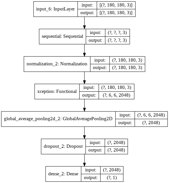
visualize the structure of the model as below:

keras.utils.plot_model(model, show_shapes=True)
plt.savefig("/content/drive/My Drive/Colab Notebooks/ComputerVision/image4.png")

png

5. Correct for data imbalance

We saw earlier in this notebook that the data was imbalanced, with more images classified as pneumonia than normal. We will correct for that in this following section.

print(Counter(train_labels)['NORMAL'])
print(Counter(train_labels)['PNEUMONIA'])


initial_bias = np.log([Counter(train_labels)['PNEUMONIA']/Counter(train_labels)['NORMAL']])
initial_bias

1341
3875

array([1.06113006])

Adjust The Model for data imbalance

There is 3875 Pneumonia exapmples compared to 1341 normal examples. The dataset highly imbalanced towards the pneumonia cases. The model has to be adjusted to reduce the biase introduced by this class imbalance.

# Scaling by total/2 can keep the loss to a similar magnitude.
# The sum of the weights of all examples stays the same.
weight_for_0 = (1 / Counter(train_labels)['NORMAL'])*(len(train_labels))/2.0 
weight_for_1 = (1 / Counter(train_labels)['PNEUMONIA'])*(len(train_labels))/2.0

class_weight = {0: weight_for_0, 1: weight_for_1}

print('Weight for class 0: {:.2f}'.format(weight_for_0))
print('Weight for class 1: {:.2f}'.format(weight_for_1))

Weight for class 0: 1.94
Weight for class 1: 0.67

set up the checkpoint to save the model at various epochs during training

import os
# Include the epoch in the file name (uses `str.format`)
#checkpoint_path = "training_2/cp-{epoch:04d}.ckpt"
#checkpoint_dir = os.path.dirname(checkpoint_path)



checkpoint_p= "/content/drive/My Drive/Colab Notebooks/ComputerVision/"
checkpoint_path = os.path.join(checkpoint_p, "cp.ckpt")
checkpoint_dir = os.path.dirname(checkpoint_path)

# Create a callback that saves the model's weights
cp_callback = tf.keras.callbacks.ModelCheckpoint(filepath=checkpoint_path,
                                                 save_weights_only=True,
                                                 monitor='val_auc',
                                                 save_best_only=True,
                                                 save_freq=10,
                                                verbose=0 )

# Keep only a single checkpoint, the best over test accuracy.
#cp_callback  = tf.keras.callbacks.ModelCheckpoint(filepath=checkpoint_path,
#                            monitor='val_accuracy',
#                            verbose=0,
#                            save_best_only=True,
#                            mode='max')


epochs = 60 

#verbose =2 print a lot of information
early_stopping_monitor = tf.keras.callbacks.EarlyStopping(patience = 20 ,
                                                          monitor = "val_auc", 
                                                        mode="max",
                                                          verbose = 0,
                                                          restore_best_weights=True)
# Train the model with the new callback
history = model.fit(train_ds, 
          #train_labels,  
          epochs=epochs,
          class_weight=class_weight,
           #steps_per_epoch= len(train_filenames)// batch_size, #run out of data
          #validation_data=(test_images,test_labels),
          validation_data=val_ds,
          verbose=1,
          callbacks=[cp_callback,early_stopping_monitor])  # Pass callback to training

Epoch 41/60
  9/131 [=>............................] - ETA: 10s - loss: 0.4795 - tp: 113.3333 - fp: 0.0000e+00 - tn: 37.3333 - fn: 9.3333 - accuracy: 0.9323 - precision: 1.0000 - recall: 0.9136 - auc: 0.9911WARNING:tensorflow:Can save best model only with val_auc available, skipping.
 19/131 [===>..........................] - ETA: 9s - loss: 0.4905 - tp: 227.2632 - fp: 0.2632 - tn: 76.1579 - fn: 16.3158 - accuracy: 0.9416 - precision: 0.9993 - recall: 0.9249 - auc: 0.9901WARNING:tensorflow:Can save best model only with val_auc available, skipping.
 29/131 [=====>........................] - ETA: 8s - loss: 0.4945 - tp: 341.5517 - fp: 0.7931 - tn: 114.9310 - fn: 22.7241 - accuracy: 0.9456 - precision: 0.9985 - recall: 0.9306 - auc: 0.9896WARNING:tensorflow:Can save best model only with val_auc available, skipping.
 39/131 [=======>......................] - ETA: 7s - loss: 0.4954 - tp: 456.8974 - fp: 1.2564 - tn: 152.4359 - fn: 29.4103 - accuracy: 0.9476 - precision: 0.9980 - recall: 0.9334 - auc: 0.9896WARNING:tensorflow:Can save best model only with val_auc available, skipping.
 49/131 [==========>...................] - ETA: 7s - loss: 0.4967 - tp: 572.1429 - fp: 1.9388 - tn: 190.9796 - fn: 34.9388 - accuracy: 0.9495 - precision: 0.9975 - recall: 0.9363 - auc: 0.9899WARNING:tensorflow:Can save best model only with val_auc available, skipping.
 59/131 [============>.................] - ETA: 6s - loss: 0.4985 - tp: 686.3220 - fp: 2.6102 - tn: 230.6271 - fn: 40.4407 - accuracy: 0.9509 - precision: 0.9971 - recall: 0.9384 - auc: 0.9899WARNING:tensorflow:Can save best model only with val_auc available, skipping.
 69/131 [==============>...............] - ETA: 5s - loss: 0.5007 - tp: 799.2899 - fp: 3.2464 - tn: 272.0145 - fn: 45.4493 - accuracy: 0.9523 - precision: 0.9969 - recall: 0.9403 - auc: 0.9899WARNING:tensorflow:Can save best model only with val_auc available, skipping.
 79/131 [=================>............] - ETA: 4s - loss: 0.5027 - tp: 911.8481 - fp: 3.7215 - tn: 313.9620 - fn: 50.4684 - accuracy: 0.9534 - precision: 0.9967 - recall: 0.9418 - auc: 0.9900WARNING:tensorflow:Can save best model only with val_auc available, skipping.
 89/131 [===================>..........] - ETA: 3s - loss: 0.5048 - tp: 1023.2022 - fp: 4.1236 - tn: 356.7865 - fn: 55.8876 - accuracy: 0.9543 - precision: 0.9967 - recall: 0.9428 - auc: 0.9900WARNING:tensorflow:Can save best model only with val_auc available, skipping.
 99/131 [=====================>........] - ETA: 2s - loss: 0.5064 - tp: 1134.9899 - fp: 4.6061 - tn: 399.2424 - fn: 61.1616 - accuracy: 0.9550 - precision: 0.9966 - recall: 0.9437 - auc: 0.9899WARNING:tensorflow:Can save best model only with val_auc available, skipping.
109/131 [=======================>......] - ETA: 1s - loss: 0.5077 - tp: 1247.1101 - fp: 5.0275 - tn: 441.2661 - fn: 66.5963 - accuracy: 0.9556 - precision: 0.9965 - recall: 0.9444 - auc: 0.9898WARNING:tensorflow:Can save best model only with val_auc available, skipping.
119/131 [==========================>...] - ETA: 1s - loss: 0.5086 - tp: 1360.1008 - fp: 5.5042 - tn: 482.6218 - fn: 71.7731 - accuracy: 0.9561 - precision: 0.9965 - recall: 0.9451 - auc: 0.9898WARNING:tensorflow:Can save best model only with val_auc available, skipping.
129/131 [============================>.] - ETA: 0s - loss: 0.5093 - tp: 1473.6047 - fp: 5.9302 - tn: 523.6512 - fn: 76.8140 - accuracy: 0.9566 - precision: 0.9965 - recall: 0.9458 - auc: 0.9897WARNING:tensorflow:Can save best model only with val_auc available, skipping.
131/131 [==============================] - 14s 108ms/step - loss: 0.5095 - tp: 1507.2424 - fp: 6.0455 - tn: 535.8712 - fn: 78.3106 - accuracy: 0.9568 - precision: 0.9965 - recall: 0.9459 - auc: 0.9897 - val_loss: 0.4360 - val_tp: 725.0000 - val_fp: 10.0000 - val_tn: 258.0000 - val_fn: 50.0000 - val_accuracy: 0.9425 - val_precision: 0.9864 - val_recall: 0.9355 - val_auc: 0.9841

#def plot_loss(history, label, n):
  # Use a log scale to show the wide range of values.
#  plt.plot(history.epoch,  history.history['loss'],
#               color=colors[n], label='Train_loss '+label)
#  plt.plot(history.epoch,  history.history['val_loss'],
 #         color=colors[n+1], label='Val_loss '+label,
 #         linestyle="--")
 # plt.xlabel('Epoch')
 # plt.ylabel('Loss')
 # plt.legend()
  #plt.savefig('acc.png')
model.save('/content/drive/My Drive/Colab Notebooks/ComputerVision/normlayer_model.h5')

# restoring the latest checkpoint in checkpoint_dir
#checkpoint.restore(tf.train.latest_checkpoint(checkpoint_path))
latest = tf.train.latest_checkpoint("/content/drive/My Drive/Colab Notebooks/ComputerVision/TrainedModel/")
# Create a new model instance
model = create_model()

# Load the previously saved weights
model.load_weights(latest)

<tensorflow.python.training.tracking.util.CheckpointLoadStatus at 0x7fc125a832b0>

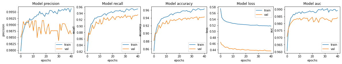
fig, ax = plt.subplots(1, 5, figsize=(20, 3))
ax = ax.ravel()

for i, met in enumerate(['precision', 'recall', 'accuracy', 'loss','auc']):
    ax[i].plot(history.history[met])
    ax[i].plot(history.history['val_' + met])
    ax[i].set_title('Model {}'.format(met))
    ax[i].set_xlabel('epochs')
    ax[i].set_ylabel(met)
    ax[i].legend(['train', 'val'])


plt.savefig("/content/drive/My Drive/Colab Notebooks/ComputerVision/image5.png")    

png

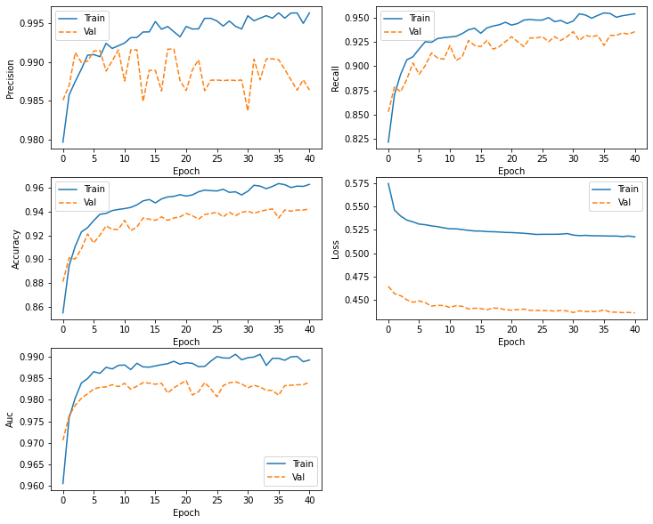
def plot_metrics(history):
  mpl.rcParams['figure.figsize'] = (12, 10)
  colors = plt.rcParams['axes.prop_cycle'].by_key()['color']  
  #metrics =  ['loss', 'auc', 'precision', 'recall']
  metrics =['precision', 'recall', 'accuracy', 'loss','auc']
  for n, metric in enumerate(metrics):
    name = metric.replace("_"," ").capitalize()
    plt.subplot(3,2,n+1)
    plt.plot(history.epoch,  history.history[metric], color=colors[0], label='Train')
    plt.plot(history.epoch, history.history['val_'+metric],
             color=colors[1], linestyle="--", label='Val')
    plt.xlabel('Epoch')
    plt.ylabel(name)
    #if metric == 'loss':
    #  plt.ylim([0, plt.ylim()[1]])
    #elif metric == 'auc':
    #  plt.ylim([0.8,1])
    #else:
    #  plt.ylim([0,1])

    plt.legend()

plot_metrics(history )
plt.savefig("/content/drive/My Drive/Colab Notebooks/ComputerVision/image6.png")  

png

# Evaluate the restored model on the valdatio set
loss,tp,fp,tn,fn,accuracy,precision,recall,auc = model.evaluate(val_ds, verbose=2)
print(' model accuracy: {:5.2f}%'.format(100*accuracy))
print(' model AUC: {:5.2f}%'.format(100*auc))

33/33 - 3s - loss: 0.4388 - tp: 721.0000 - fp: 10.0000 - tn: 258.0000 - fn: 54.0000 - accuracy: 0.9386 - precision: 0.9863 - recall: 0.9303 - auc: 0.9844
 model accuracy: 93.86%
 model accuracy: 98.44%

#loss, acc = new_model.evaluate(test_images,  test_labels, verbose=2)
#loss, acc = model.evaluate(val_ds, verbose=2)
#print('Restored model, accuracy: {:5.2f}%'.format(100*acc))

#print(new_model.predict(test_images).shape)

predictions = model.predict(test_ds, batch_size=batch_size)


test_labels_num =  [1 if x =='PNEUMONIA' else 0 for x in test_labels]

from sklearn.metrics import classification_report
from sklearn.metrics import confusion_matrix
import seaborn as sns
p=0.5

def PlotConfusionMatrix(y_test,pred,y_test_normal,y_test_pneumonia,label):

    cfn_matrix = confusion_matrix(y_test,pred)
    cfn_norm_matrix = np.array([[1.0 / y_test_normal,1.0/y_test_normal],[1.0/y_test_pneumonia,1.0/y_test_pneumonia]])
    norm_cfn_matrix = cfn_matrix * cfn_norm_matrix

    #colsum=cfn_matrix.sum(axis=0)
    #norm_cfn_matrix = cfn_matrix / np.vstack((colsum, colsum)).T

    fig = plt.figure(figsize=(15,5))
    ax = fig.add_subplot(1,2,1)
    sns.heatmap(cfn_matrix,cmap='magma',linewidths=0.5,annot=True,ax=ax)
    #tick_marks = np.arange(len(y_test))
    #plt.xticks(tick_marks, np.unique(y_test), rotation=45)
    plt.title('Confusion Matrix',color='b')
    plt.ylabel('Real Classes')
    plt.xlabel('Predicted Classes')
    plt.savefig('/content/drive/My Drive/Colab Notebooks/ComputerVision/cm_' +label +  '.png')
        
    ax = fig.add_subplot(1,2,2)
    sns.heatmap(norm_cfn_matrix,cmap=plt.cm.Blues,linewidths=0.5,annot=True,ax=ax)

    plt.title('Normalized Confusion Matrix',color='b')
    plt.ylabel('Real Classes')
    plt.xlabel('Predicted Classes')
    plt.savefig('/content/drive/My Drive/Colab Notebooks/ComputerVision/cm_norm' +label +  '.png')
    plt.show()
    
    print('---Classification Report---')
    print(classification_report(y_test,pred))
    

y_test_normal,y_test_pneumonia = np.bincount(test_labels_num)
y_pred= np.where(predictions<p,0,1 )


PlotConfusionMatrix(test_labels_num,y_pred,y_test_normal,y_test_pneumonia,label='pneumonia classification')

png

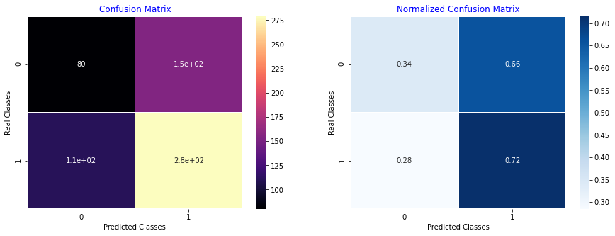
---Classification Report---
              precision    recall  f1-score   support

           0       0.42      0.34      0.38       234
           1       0.64      0.72      0.68       390

    accuracy                           0.58       624
   macro avg       0.53      0.53      0.53       624
weighted avg       0.56      0.58      0.56       624

# check the checkpoint directory
!ls {checkpoint_dir}

ls: cannot access '{checkpoint_dir}': No such file or directory

Predict and evaluate results

Let’s evaluate the model on our test data!

#loss, acc, prec, rec = model.evaluate(test_ds)

# Evaluate the restored model on the test set
loss,tp,fp,tn,fn,accuracy,precision,recall,auc =  model.evaluate(test_ds, verbose=2)
print(' model accuracy: {:5.2f}%'.format(100*accuracy))
print(' area under the  roc curve: {:5.2f}%'.format(100*auc))

20/20 - 5s - loss: 0.5239 - tp: 375.0000 - fp: 58.0000 - tn: 176.0000 - fn: 15.0000 - accuracy: 0.8830 - precision: 0.8661 - recall: 0.9615 - auc: 0.9402
 model accuracy: 88.30%
 area under the  roc curve: 94.02%

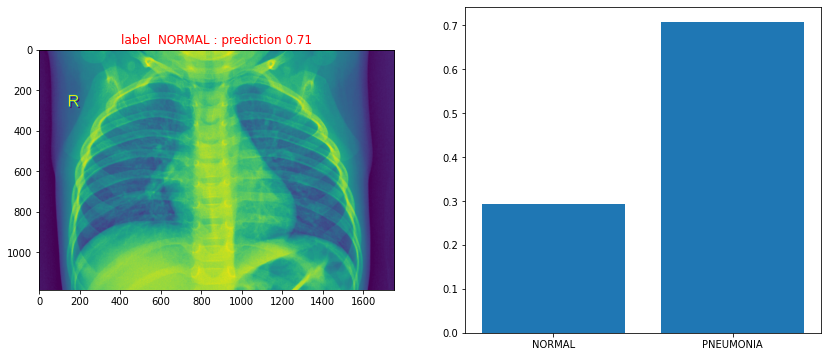
#randomly sample an image from the test set and predict it's label
path=[test_filenames[i] for i in np.random.randint(len(test_filenames), size=1)][0]
print(path)
# Loads an image into PIL format.
tf.keras.preprocessing.image.load_img(
    path, grayscale=False, color_mode="rgb", target_size=None, interpolation="bilinear")


image = tf.keras.preprocessing.image.load_img(path, interpolation="bilinear")
input_arr = keras.preprocessing.image.img_to_array(image)
input_arr = np.array([input_arr])  # Convert single image to a batch.
prediction = model.predict(input_arr,batch_size=batch_size)
label =["PNEUMONIA" if "PNEUMONIA" in path else "NORMAL"]
predicted_label =["PNEUMONIA" if prediction > 0.5 else "NORMAL"]
#predicted_label
print("True label  {n} : predicted probability {s}: predicted label {l}".format(n=label[0], s=prediction[0][0],l=predicted_label[0]))  

chest_xray/chest_xray/test/NORMAL/IM-0084-0001.jpeg
WARNING:tensorflow:Model was constructed with shape (None, 180, 180, 3) for input KerasTensor(type_spec=TensorSpec(shape=(None, 180, 180, 3), dtype=tf.float32, name='input_6'), name='input_6', description="Symbolic value 0 from symbolic call 0 of layer 'input_6'"), but it was called on an input with incompatible shape (None, 1187, 1754, 3).
WARNING:tensorflow:Model was constructed with shape (None, 180, 180, 3) for input KerasTensor(type_spec=TensorSpec(shape=(None, 180, 180, 3), dtype=tf.float32, name='input_5'), name='input_5', description="Symbolic value 0 from symbolic call 0 of layer 'input_5'"), but it was called on an input with incompatible shape (None, 1187, 1754, 3).
True label  NORMAL : predicted probability 0.7068414092063904: predicted label PNEUMONIA

To upload a single image and predict with the model, you can try the following:

import numpy as np
from google.colab import files
from keras.preprocessing import image

uploaded = files.upload()

for fn in uploaded.keys():
 
  # predicting images
  path = fn
  img = image.load_img(path, target_size=(150, 150))
  x = image.img_to_array(img)
  x = np.expand_dims(x, axis=0)

  images = np.vstack([x])
  classes = model.predict(images, batch_size=batch_size)
  print(fn)
  print(classes)

 <input type="file" id="files-2d57ae01-61bd-42c2-a755-88cc4d7fcc9e" name="files[]" multiple disabled
    style="border:none" />
 <output id="result-2d57ae01-61bd-42c2-a755-88cc4d7fcc9e">
  Upload widget is only available when the cell has been executed in the
  current browser session. Please rerun this cell to enable.
  </output>
  <script src="/nbextensions/google.colab/files.js"></script> 


Saving datasets_17810_23812_chest_xray_val_NORMAL_NORMAL2-IM-1430-0001.jpeg to datasets_17810_23812_chest_xray_val_NORMAL_NORMAL2-IM-1430-0001.jpeg
datasets_17810_23812_chest_xray_val_NORMAL_NORMAL2-IM-1430-0001.jpeg
[[0.9991202]]

%pylab inline
import matplotlib.pyplot as plt
import matplotlib.image as mpimg
img=mpimg.imread(path)

#fig, axs = plt.subplots(1,2, figsize=(15, 6), facecolor='w', edgecolor='k')
fig.subplots_adjust(hspace = .5, wspace=.001)
fig, (ax1, ax2) = plt.subplots(1, 2, figsize=(14, 6), facecolor='w', edgecolor='k')
#axs = axs.ravel()

ax1.imshow(mpimg.imread(path))
ax1.set_title("label  {} : prediction {:0.2f}".format(label[0], prediction[0][0] ),color='r')
#ax1.set_title("%.2f kg = %.2f lb = %.2f gal = %.2f l" % (label[0], prediction[0][0] )
#axs[i].set_title(label[i])
ax2.bar([0,1],[1-prediction[0][0],prediction[0][0]])
plt.xticks([0,1], ('NORMAL', 'PNEUMONIA'))
plt.plot()
plt.show()
plt.savefig("/content/drive/My Drive/Colab Notebooks/ComputerVision/image7.png") 

Populating the interactive namespace from numpy and matplotlib

png

<Figure size 432x288 with 0 Axes>

Fine-tuning

We can approach fine-tuning by unfreezing all or part of the base model and retrain the whole model end-to-end with a very low learning rate after the model has converged. Fine-tuning can lead to model performance improvement wheras at the same time it can easily lead to overfitting. It is critically important to use a very low learning rate at this stage, because you are training a much larger model than in the first round of training, on a small dataset.

def finetune_model():
    base_model = tf.keras.applications.Xception(
    weights="imagenet",  # Load weights pre-trained on ImageNet.
    input_shape=input_shape,
    include_top=False,
     )  # Do not include the ImageNet classifier at the top.

# Unfreeze the base_model. Note that it keeps running in inference mode
# since we passed `training=False` when calling it. This means that
# the batchnorm layers will not update their batch statistics.
# This prevents the batchnorm layers from undoing all the training
# we've done so far.
    base_model.trainable = True
    optimizer=tf.keras.optimizers.Adam(1e-5)
# Create new model on top
    inputs = tf.keras.Input(shape=input_shape)
    x = data_augmentation(inputs)  # Apply random data augmentation

# Pre-trained Xception weights requires that input be normalized
# from (0, 255) to a range (-1., +1.), the normalization layer
#  does the following, outputs = (inputs - mean) / sqrt(var)
    norm_layer = tf.keras.layers.experimental.preprocessing.Normalization()
    mean = np.array([127.5] * 3)
    var = mean ** 2
# Scale inputs to [-1, +1]
    x = norm_layer(x)
    norm_layer.set_weights([mean, var])

# The base model contains batchnorm layers. We want to keep them in inference mode
# when we unfreeze the base model for fine-tuning, so we make sure that the
# base_model is running in inference mode here.
    x = base_model(x, training=False)
    x = keras.layers.GlobalAveragePooling2D()(x)
    x = keras.layers.Dropout(0.2)(x)  # Regularize with dropout
    # A Dense classifier with a single unit (binary classification)
    outputs = tf.keras.layers.Dense(units=num_classes, activation = 'sigmoid')(x)
    model = tf.keras.Model(inputs, outputs)
    model.compile(optimizer=optimizer,
              loss=keras.losses.BinaryCrossentropy(from_logits=True),
              metrics=METRICS)  #[keras.metrics.BinaryAccuracy()]
    return model

# Create a basic model instance
model = finetune_model()

# Display the model's architecture
model.summary()

Model: "functional_7"
_________________________________________________________________
Layer (type)                 Output Shape              Param #   
=================================================================
input_8 (InputLayer)         [(None, 180, 180, 3)]     0         
_________________________________________________________________
sequential (Sequential)      (None, None, None, 3)     0         
_________________________________________________________________
normalization_3 (Normalizati (None, 180, 180, 3)       7         
_________________________________________________________________
xception (Functional)        (None, 6, 6, 2048)        20861480  
_________________________________________________________________
global_average_pooling2d_3 ( (None, 2048)              0         
_________________________________________________________________
dropout_3 (Dropout)          (None, 2048)              0         
_________________________________________________________________
dense_3 (Dense)              (None, 1)                 2049      
=================================================================
Total params: 20,863,536
Trainable params: 20,809,001
Non-trainable params: 54,535
_________________________________________________________________

import os
# Include the epoch in the file name (uses `str.format`)
#checkpoint_path = "training_2/cp-{epoch:04d}.ckpt"
#checkpoint_dir = os.path.dirname(checkpoint_path)



checkpoint_p= "/content/drive/My Drive/Colab Notebooks/ComputerVision/"
checkpoint_path = os.path.join(checkpoint_p, "cp.ckpt")
checkpoint_dir = os.path.dirname(checkpoint_path)

# Create a callback that saves the model's weights
# Keep only a single checkpoint, the best over validation accuracy.
cp_callback = tf.keras.callbacks.ModelCheckpoint(filepath=checkpoint_path,
                                                 save_weights_only=True,
                                                 monitor='val_auc',
                                                 save_best_only=True,
                                                 save_freq=10,
                                                verbose=0 )


#cp_callback  = tf.keras.callbacks.ModelCheckpoint(filepath=checkpoint_path,
#                            monitor='val_accuracy',
#                            verbose=0,
#                            save_best_only=True,
#                            mode='max')


epochs = 100 

#verbose =2 print a lot of information
early_stopping_monitor = tf.keras.callbacks.EarlyStopping(patience = 30 ,
                                                          monitor = "val_auc", 
                                                        mode="max",
                                                          verbose = 1,
                                                          restore_best_weights=True)
# Train the model with the new callback
history = model.fit(train_ds, 
          #train_labels,  
          epochs=epochs,
          class_weight=class_weight,
           #steps_per_epoch= len(train_filenames)// batch_size, #run out of data
          #validation_data=(test_images,test_labels),
          validation_data=val_ds,
          verbose=1,
          callbacks=[cp_callback,early_stopping_monitor])  # Pass callback to training

WARNING:tensorflow:Automatic model reloading for interrupted job was removed from the `ModelCheckpoint` callback in multi-worker mode, please use the `keras.callbacks.experimental.BackupAndRestore` callback instead. See this tutorial for details: https://www.tensorflow.org/tutorials/distribute/multi_worker_with_keras#backupandrestore_callback.
Epoch 1/100
  9/131 [=>............................] - ETA: 2:05 - loss: 0.6876 - tp: 488.2222 - fp: 89.8889 - tn: 181.4444 - fn: 24.4444 - accuracy: 0.8553 - precision: 0.8455 - recall: 0.9527 - auc: 0.8998WARNING:tensorflow:Can save best model only with val_auc available, skipping.  .  .  .
   
Epoch 32/100
  8/131 [>.............................] - ETA: 48s - loss: 0.4593 - tp: 111.0000 - fp: 0.0000e+00 - tn: 33.0000 - fn: 0.0000e+00 - accuracy: 1.0000 - precision: 1.0000 - recall: 1.0000 - auc: 1.0000WARNING:tensorflow:Can save best model only with val_auc available, skipping.
 18/131 [===>..........................] - ETA: 44s - loss: 0.4746 - tp: 230.8889 - fp: 0.0000e+00 - tn: 72.6111 - fn: 0.5000 - accuracy: 0.9988 - precision: 1.0000 - recall: 0.9985 - auc: 0.9992WARNING:tensorflow:Can save best model only with val_auc available, skipping.
 28/131 [=====>........................] - ETA: 40s - loss: 0.4790 - tp: 351.4643 - fp: 0.0000e+00 - tn: 111.8571 - fn: 0.6786 - accuracy: 0.9988 - precision: 1.0000 - recall: 0.9984 - auc: 0.9992WARNING:tensorflow:Can save best model only with val_auc available, skipping.
 38/131 [=======>......................] - ETA: 36s - loss: 0.4801 - tp: 473.3421 - fp: 0.0000e+00 - tn: 149.8947 - fn: 0.7632 - accuracy: 0.9988 - precision: 1.0000 - recall: 0.9985 - auc: 0.9992WARNING:tensorflow:Can save best model only with val_auc available, skipping.
 48/131 [=========>....................] - ETA: 32s - loss: 0.4814 - tp: 594.3125 - fp: 0.0000e+00 - tn: 188.8750 - fn: 0.8125 - accuracy: 0.9989 - precision: 1.0000 - recall: 0.9986 - auc: 0.9993WARNING:tensorflow:Can save best model only with val_auc available, skipping.
 58/131 [============>.................] - ETA: 28s - loss: 0.4831 - tp: 713.8621 - fp: 0.0000e+00 - tn: 229.1379 - fn: 1.0000 - accuracy: 0.9989 - precision: 1.0000 - recall: 0.9986 - auc: 0.9993WARNING:tensorflow:Can save best model only with val_auc available, skipping.
 68/131 [==============>...............] - ETA: 24s - loss: 0.4854 - tp: 831.8824 - fp: 0.0000e+00 - tn: 270.9559 - fn: 1.1618 - accuracy: 0.9989 - precision: 1.0000 - recall: 0.9986 - auc: 0.9993WARNING:tensorflow:Can save best model only with val_auc available, skipping.
 78/131 [================>.............] - ETA: 20s - loss: 0.4875 - tp: 949.1410 - fp: 0.0000e+00 - tn: 313.4103 - fn: 1.4487 - accuracy: 0.9989 - precision: 1.0000 - recall: 0.9985 - auc: 0.9993WARNING:tensorflow:Can save best model only with val_auc available, skipping.
 88/131 [===================>..........] - ETA: 17s - loss: 0.4897 - tp: 1065.5909 - fp: 0.0000e+00 - tn: 356.5568 - fn: 1.8523 - accuracy: 0.9988 - precision: 1.0000 - recall: 0.9984 - auc: 0.9992WARNING:tensorflow:Can save best model only with val_auc available, skipping.
 98/131 [=====================>........] - ETA: 13s - loss: 0.4914 - tp: 1182.2041 - fp: 0.0000e+00 - tn: 399.5816 - fn: 2.2143 - accuracy: 0.9987 - precision: 1.0000 - recall: 0.9983 - auc: 0.9992WARNING:tensorflow:Can save best model only with val_auc available, skipping.
108/131 [=======================>......] - ETA: 9s - loss: 0.4928 - tp: 1299.2778 - fp: 0.0000e+00 - tn: 442.0741 - fn: 2.6481 - accuracy: 0.9987 - precision: 1.0000 - recall: 0.9982 - auc: 0.9991WARNING:tensorflow:Can save best model only with val_auc available, skipping.
118/131 [==========================>...] - ETA: 5s - loss: 0.4938 - tp: 1417.0424 - fp: 0.0508 - tn: 483.8898 - fn: 3.0169 - accuracy: 0.9986 - precision: 1.0000 - recall: 0.9981 - auc: 0.9990WARNING:tensorflow:Can save best model only with val_auc available, skipping.
128/131 [============================>.] - ETA: 1s - loss: 0.4946 - tp: 1535.2344 - fp: 0.1250 - tn: 525.3125 - fn: 3.3281 - accuracy: 0.9986 - precision: 1.0000 - recall: 0.9981 - auc: 0.9990WARNING:tensorflow:Can save best model only with val_auc available, skipping.
131/131 [==============================] - ETA: 0s - loss: 0.4948 - tp: 1570.5725 - fp: 0.1450 - tn: 537.7176 - fn: 3.4198 - accuracy: 0.9985 - precision: 0.9999 - recall: 0.9981 - auc: 0.9990Restoring model weights from the end of the best epoch.
131/131 [==============================] - 55s 416ms/step - loss: 0.4949 - tp: 1582.0985 - fp: 0.1515 - tn: 541.7652 - fn: 3.4545 - accuracy: 0.9985 - precision: 0.9999 - recall: 0.9981 - auc: 0.9990 - val_loss: 0.4188 - val_tp: 766.0000 - val_fp: 8.0000 - val_tn: 260.0000 - val_fn: 9.0000 - val_accuracy: 0.9837 - val_precision: 0.9897 - val_recall: 0.9884 - val_auc: 0.9882
Epoch 00032: early stopping

The results from finetuning does not show an improvement. The model actually deteriorates after finetuning.

# Evaluate the restored model on the valdatio set
loss,tp,fp,tn,fn,accuracy,precision,recall,auc = model.evaluate(test_ds, verbose=2)
print(' model accuracy: {:5.2f}%'.format(100*accuracy))
print(' model AUC: {:5.2f}%'.format(100*auc))

20/20 - 5s - loss: 0.5536 - tp: 385.0000 - fp: 96.0000 - tn: 138.0000 - fn: 5.0000 - accuracy: 0.8381 - precision: 0.8004 - recall: 0.9872 - auc: 0.8938
 model accuracy: 83.81%
 model accuracy: 89.38%

The fine-tuned model save can be saved to file and loaded for later use. The fine-tuning resulted in a weaker model performance than expected, the hope with fine-tuning a model is to try to improve the performance of the model but in this case we were not able to do that.

model.save('/content/drive/My Drive/Colab Notebooks/ComputerVision/pneumoniafinetuned/finetuned_model2.h5')
# Recreate the exact same model purely from the file
#new_model = tf.keras.models.load_model('/finetuned_model2.h5')

cp_callback = tf.keras.callbacks.ModelCheckpoint("/content/drive/My Drive/Colab Notebooks/ComputerVision/pneumoniatrainmodel/normlayer_model.h5",
                                                    save_best_only=True)

early_stopping_monitor = tf.keras.callbacks.EarlyStopping(patience=30,
                                                     restore_best_weights=True)