Automatic Machine Learning

Automated Machine Learning

Automated Machine Learning (AutoML) has increased greatly the efficiency of building machine learning models. AutoML achieves this by automating in some applications data pre-processing ,feature engineering, feature extraction , feature selection and hyper-parameter tuning when building machine learning models. AutoML has also reduced the expertise in academic domains such as computer science, statistics and other academic knowledge hitherto needed to build machine learning models. Repetitive task which do not need any expertise in machine learning could be easily automated by AutoML. AutoML can have some drawback which include the amount of time used in training. Since AutoML trains many models and selects the best performing model as the final model, large computaional resources is needed to reduce the time involved in training.

Data

Appliances energy prediction dataset from UCI machine learning repository would be used for this exercise. Further description of data and the data itself is available here. The goal is to predict home Appliance energy use in Wh given several features including temperature in various rooms of the house and humidity etc.

Attribute Information:

date time year-month-day hour:minute:second
Appliances, energy use in Wh lights, energy use of light fixtures in the house in Wh
T1, Temperature in kitchen area, in Celsius
RH_1, Humidity in kitchen area, in %
T2, Temperature in living room area, in Celsius
RH_2, Humidity in living room area, in %
T3, Temperature in laundry room area
RH_3, Humidity in laundry room area, in %
T4, Temperature in office room, in Celsius
RH_4, Humidity in office room, in %
T5, Temperature in bathroom, in Celsius
RH_5, Humidity in bathroom, in %
T6, Temperature outside the building (north side), in Celsius
RH_6, Humidity outside the building (north side), in %
T7, Temperature in ironing room , in Celsius
RH_7, Humidity in ironing room, in %
T8, Temperature in teenager room 2, in Celsius
RH_8, Humidity in teenager room 2, in %
T9, Temperature in parents room, in Celsius
RH_9, Humidity in parents room, in %
To, Temperature outside (from Chievres weather station), in Celsius
Pressure (from Chievres weather station), in mm Hg
RH_out, Humidity outside (from Chievres weather station), in %
Wind speed (from Chievres weather station), in m/s
Visibility (from Chievres weather station), in km
Tdewpoint (from Chievres weather station), Â°C
rv1, Random variable 1, nondimensional
rv2, Random variable 2, nondimensional

import numpy as np
import pandas as pd
from google.colab import files
import io
from sklearn.model_selection import train_test_split
import rpy2
%load_ext rpy2.ipython

The rpy2.ipython extension is already loaded. To reload it, use:
  %reload_ext rpy2.ipython

uploaded = files.upload()

 <input type="file" id="files-5333c190-8c44-4f40-82a7-fbb1943d7fea" name="files[]" multiple disabled />
 <output id="result-5333c190-8c44-4f40-82a7-fbb1943d7fea">
  Upload widget is only available when the cell has been executed in the
  current browser session. Please rerun this cell to enable.
  </output>
  <script src="/nbextensions/google.colab/files.js"></script> 


Saving energydata_complete.csv to energydata_complete.csv

for fn in uploaded.keys():
  print('User uploaded file "{name}" with length {length} bytes'.format(
      name=fn, length=len(uploaded[fn])))

User uploaded file "energydata_complete.csv" with length 11979363 bytes

dateparse = lambda x: pd.datetime.strptime(x, '%Y-%m-%d %H:%M:%S')

energy_data=pd.read_csv(io.StringIO(uploaded['energydata_complete.csv'].decode('utf-8')),
                        parse_dates=['date'], 
                        date_parser=dateparse)
energy_data.head()

	date	Appliances	lights	T1	RH_1	T2	RH_2	T3	RH_3	T4	RH_4	T5	RH_5	T6	RH_6	T7	RH_7	T8	RH_8	T9	RH_9	T_out	Press_mm_hg	RH_out	Windspeed	Visibility	Tdewpoint	rv1	rv2
0	2016-01-11 17:00:00	60	30	19.89	47.596667	19.2	44.790000	19.79	44.730000	19.000000	45.566667	17.166667	55.20	7.026667	84.256667	17.200000	41.626667	18.2	48.900000	17.033333	45.53	6.600000	733.5	92.0	7.000000	63.000000	5.3	13.275433	13.275433
1	2016-01-11 17:10:00	60	30	19.89	46.693333	19.2	44.722500	19.79	44.790000	19.000000	45.992500	17.166667	55.20	6.833333	84.063333	17.200000	41.560000	18.2	48.863333	17.066667	45.56	6.483333	733.6	92.0	6.666667	59.166667	5.2	18.606195	18.606195
2	2016-01-11 17:20:00	50	30	19.89	46.300000	19.2	44.626667	19.79	44.933333	18.926667	45.890000	17.166667	55.09	6.560000	83.156667	17.200000	41.433333	18.2	48.730000	17.000000	45.50	6.366667	733.7	92.0	6.333333	55.333333	5.1	28.642668	28.642668
3	2016-01-11 17:30:00	50	40	19.89	46.066667	19.2	44.590000	19.79	45.000000	18.890000	45.723333	17.166667	55.09	6.433333	83.423333	17.133333	41.290000	18.1	48.590000	17.000000	45.40	6.250000	733.8	92.0	6.000000	51.500000	5.0	45.410389	45.410389
4	2016-01-11 17:40:00	60	40	19.89	46.333333	19.2	44.530000	19.79	45.000000	18.890000	45.530000	17.200000	55.09	6.366667	84.893333	17.200000	41.230000	18.1	48.590000	17.000000	45.40	6.133333	733.9	92.0	5.666667	47.666667	4.9	10.084097	10.084097

energy_data.info()

<class 'pandas.core.frame.DataFrame'>
RangeIndex: 19735 entries, 0 to 19734
Data columns (total 29 columns):
date           19735 non-null datetime64[ns]
Appliances     19735 non-null int64
lights         19735 non-null int64
T1             19735 non-null float64
RH_1           19735 non-null float64
T2             19735 non-null float64
RH_2           19735 non-null float64
T3             19735 non-null float64
RH_3           19735 non-null float64
T4             19735 non-null float64
RH_4           19735 non-null float64
T5             19735 non-null float64
RH_5           19735 non-null float64
T6             19735 non-null float64
RH_6           19735 non-null float64
T7             19735 non-null float64
RH_7           19735 non-null float64
T8             19735 non-null float64
RH_8           19735 non-null float64
T9             19735 non-null float64
RH_9           19735 non-null float64
T_out          19735 non-null float64
Press_mm_hg    19735 non-null float64
RH_out         19735 non-null float64
Windspeed      19735 non-null float64
Visibility     19735 non-null float64
Tdewpoint      19735 non-null float64
rv1            19735 non-null float64
rv2            19735 non-null float64
dtypes: datetime64[ns](1), float64(26), int64(2)
memory usage: 4.4 MB

energy_data.describe().transpose()

	count	mean	std	min	25%	50%	75%	max
Appliances	19735.0	97.694958	102.524891	10.000000	50.000000	60.000000	100.000000	1080.000000
lights	19735.0	3.801875	7.935988	0.000000	0.000000	0.000000	0.000000	70.000000
T1	19735.0	21.686571	1.606066	16.790000	20.760000	21.600000	22.600000	26.260000
RH_1	19735.0	40.259739	3.979299	27.023333	37.333333	39.656667	43.066667	63.360000
T2	19735.0	20.341219	2.192974	16.100000	18.790000	20.000000	21.500000	29.856667
RH_2	19735.0	40.420420	4.069813	20.463333	37.900000	40.500000	43.260000	56.026667
T3	19735.0	22.267611	2.006111	17.200000	20.790000	22.100000	23.290000	29.236000
RH_3	19735.0	39.242500	3.254576	28.766667	36.900000	38.530000	41.760000	50.163333
T4	19735.0	20.855335	2.042884	15.100000	19.530000	20.666667	22.100000	26.200000
RH_4	19735.0	39.026904	4.341321	27.660000	35.530000	38.400000	42.156667	51.090000
T5	19735.0	19.592106	1.844623	15.330000	18.277500	19.390000	20.619643	25.795000
RH_5	19735.0	50.949283	9.022034	29.815000	45.400000	49.090000	53.663333	96.321667
T6	19735.0	7.910939	6.090347	-6.065000	3.626667	7.300000	11.256000	28.290000
RH_6	19735.0	54.609083	31.149806	1.000000	30.025000	55.290000	83.226667	99.900000
T7	19735.0	20.267106	2.109993	15.390000	18.700000	20.033333	21.600000	26.000000
RH_7	19735.0	35.388200	5.114208	23.200000	31.500000	34.863333	39.000000	51.400000
T8	19735.0	22.029107	1.956162	16.306667	20.790000	22.100000	23.390000	27.230000
RH_8	19735.0	42.936165	5.224361	29.600000	39.066667	42.375000	46.536000	58.780000
T9	19735.0	19.485828	2.014712	14.890000	18.000000	19.390000	20.600000	24.500000
RH_9	19735.0	41.552401	4.151497	29.166667	38.500000	40.900000	44.338095	53.326667
T_out	19735.0	7.411665	5.317409	-5.000000	3.666667	6.916667	10.408333	26.100000
Press_mm_hg	19735.0	755.522602	7.399441	729.300000	750.933333	756.100000	760.933333	772.300000
RH_out	19735.0	79.750418	14.901088	24.000000	70.333333	83.666667	91.666667	100.000000
Windspeed	19735.0	4.039752	2.451221	0.000000	2.000000	3.666667	5.500000	14.000000
Visibility	19735.0	38.330834	11.794719	1.000000	29.000000	40.000000	40.000000	66.000000
Tdewpoint	19735.0	3.760707	4.194648	-6.600000	0.900000	3.433333	6.566667	15.500000
rv1	19735.0	24.988033	14.496634	0.005322	12.497889	24.897653	37.583769	49.996530
rv2	19735.0	24.988033	14.496634	0.005322	12.497889	24.897653	37.583769	49.996530

We would perform some light feature engineering by creating additional time-based features from the date column and drop the date column.

energy_data['hour']  = energy_data['date'].dt.hour
energy_data['day'] = energy_data['date'].dt.day
energy_data['month'] = pd.DatetimeIndex(energy_data['date']).month
energy_data['week'] = energy_data['date'].dt.week
energy_data['weekday']= energy_data['date'].dt.weekday
energy_data['quarter']= energy_data['date'].dt.quarter
energy_data['year'] =   pd.DatetimeIndex(energy_data['date']).year
Energy_Data = energy_data.drop(['date'],axis=1)

x= Energy_Data.drop('Appliances',axis=1)
y= Energy_Data.Appliances
train_x, test_x, train_y, test_y = train_test_split(x, y,test_size=0.3, random_state=148)

Cloud AutoML

Google Cloud AutoML is among the early implementors and also popular AutoML software around. Googles AutoML is however not open source and you need some Google account and GCP credit to train AutoML on Google cloud. Google AutoML uses neural architecture search to find a the optimal neural network architecture.

Tree-Based Pipeline Optimization Tool(TPOT)

TPOT library built on top of scikit-learn, and my favorite thing about it is that when you export a model you’re actually exporting all the Python code you need to train that model.

TPOT is a Python Automated Machine Learning tool built on top of scikit-learn ML library that optimizes machine learning pipelines using genetic programming. TPOT automates the building of ML pipelines by combining a flexible expression tree representation of pipelines with stochastic search algorithms such as genetic programming. TPOT explores thousands of possible pipelines, selects the best one for your data and finaly provides you with the python code. Both regression and classfication models can be built with TPOTRegressor and TPOTClassifier.

!conda install numpy scipy scikit-learn pandas joblib
!pip install deap update_checker tqdm stopit
!pip install xgboost
!pip install dask[delayed] dask[dataframe] dask-ml fsspec>=0.3.3
!pip install scikit-mdr skrebate
!pip install tpot
!pip install h2o

/bin/bash: conda: command not found
Collecting deap
[?25l  Downloading https://files.pythonhosted.org/packages/81/98/3166fb5cfa47bf516e73575a1515734fe3ce05292160db403ae542626b32/deap-1.3.0-cp36-cp36m-manylinux2010_x86_64.whl (151kB)

from tpot import TPOTClassifier
from tpot import TPOTRegressor
from sklearn.datasets import load_digits
from sklearn.model_selection import train_test_split

# create & fit TPOT classifier with 
pipeline_optimizer = TPOTRegressor(generations=5,
                                    population_size=20,
                                    cv=5,
                                    random_state=42,
                                    #njobs=-1,
                                    scoring= 'neg_mean_squared_error', #'f1', 'f1_macro', 'f1_micro',
                                    max_time_mins= 60,  #MAX_TIME_MINS
                                    max_eval_time_mins	=20,
                                    verbosity=2)


pipeline_optimizer.fit(train_x, train_y)
print(pipeline_optimizer.score(test_x, test_y))

HBox(children=(FloatProgress(value=0.0, description='Optimization Progress', max=20.0, style=ProgressStyle(des…


Generation 1 - Current best internal CV score: -5690.647614823849
Generation 2 - Current best internal CV score: -5690.647614823849
Generation 3 - Current best internal CV score: -5526.782440894636
Generation 4 - Current best internal CV score: -5344.624150306781


TPOT closed during evaluation in one generation.
WARNING: TPOT may not provide a good pipeline if TPOT is stopped/interrupted in a early generation.


TPOT closed prematurely. Will use the current best pipeline.

Best pipeline: RandomForestRegressor(CombineDFs(input_matrix, input_matrix), bootstrap=False, max_features=0.05, min_samples_leaf=1, min_samples_split=14, n_estimators=100)
-4983.7293780759865


/usr/local/lib/python3.6/dist-packages/sklearn/preprocessing/_function_transformer.py:97: FutureWarning: The default validate=True will be replaced by validate=False in 0.22.
  "validate=False in 0.22.", FutureWarning)
/usr/local/lib/python3.6/dist-packages/sklearn/preprocessing/_function_transformer.py:97: FutureWarning: The default validate=True will be replaced by validate=False in 0.22.
  "validate=False in 0.22.", FutureWarning)

# save our model code
#tpot.export('tpot_pipeline.py')


pipeline_optimizer.export('tpot_exported_pipeline.py')

# print the model code to see what it says
#!cat tpot_pipeline.py

predict(test_x)

H20.ai AutoML

H2O’s AutoML can be used for automating the machine learning workflow, which includes automatic training and tuning of many models within a user-specified time-limit.

H2O AutoML performs Random Search followed by a stacking stage. By default it uses the H2O machine learning package, which supports distributed training. It is available in both Python and R languages.

import h2o
from h2o.automl import H2OAutoML

# initilaize an H20 instance running locally
h2o.init(nthreads=-1)

h2o.cluster().show_status()


# convert our data to h20Frame
Energy_Data_h2o = h2o.H2OFrame(Energy_Data)



#train_data = train_data.cbind(y_data)
splits = Energy_Data_h2o.split_frame(ratios = [0.7], seed = 1)
train = splits[0]
test = splits[1]

folds = 5

# Run AutoML for 20 base models (limited to 1 hour max runtime by default)
aml = H2OAutoML(max_models=20,
                max_runtime_secs=600,
                # validation_frame=val_df,
                nfolds = folds,
                #balance_classes = TRUE, 
                stopping_metric='AUTO',  #aucpr,mean_per_class_error,logloss
                sort_metric = "RMSE",
                seed=1)
aml.train(y = 'Appliances', training_frame=train
          #leaderboard_frame = test
          )



# The leader model can be access with `aml.leader`
# save the model out (we'll need to for tomorrow!)
h2o.save_model(aml.leader)

Checking whether there is an H2O instance running at http://localhost:54321 ..... not found.
Attempting to start a local H2O server...
  Java Version: openjdk version "11.0.4" 2019-07-16; OpenJDK Runtime Environment (build 11.0.4+11-post-Ubuntu-1ubuntu218.04.3); OpenJDK 64-Bit Server VM (build 11.0.4+11-post-Ubuntu-1ubuntu218.04.3, mixed mode, sharing)
  Starting server from /usr/local/lib/python3.6/dist-packages/h2o/backend/bin/h2o.jar
  Ice root: /tmp/tmpyby0u3va
  JVM stdout: /tmp/tmpyby0u3va/h2o_unknownUser_started_from_python.out
  JVM stderr: /tmp/tmpyby0u3va/h2o_unknownUser_started_from_python.err
  Server is running at http://127.0.0.1:54321
Connecting to H2O server at http://127.0.0.1:54321 ... successful.

H2O cluster uptime:	02 secs
H2O cluster timezone:	Etc/UTC
H2O data parsing timezone:	UTC
H2O cluster version:	3.28.0.1
H2O cluster version age:	1 day
H2O cluster name:	H2O_from_python_unknownUser_dm09ir
H2O cluster total nodes:	1
H2O cluster free memory:	2.938 Gb
H2O cluster total cores:	2
H2O cluster allowed cores:	2
H2O cluster status:	accepting new members, healthy
H2O connection url:	http://127.0.0.1:54321
H2O connection proxy:	{'http': None, 'https': None}
H2O internal security:	False
H2O API Extensions:	Amazon S3, XGBoost, Algos, AutoML, Core V3, TargetEncoder, Core V4
Python version:	3.6.9 final

H2O cluster uptime:	02 secs
H2O cluster timezone:	Etc/UTC
H2O data parsing timezone:	UTC
H2O cluster version:	3.28.0.1
H2O cluster version age:	1 day
H2O cluster name:	H2O_from_python_unknownUser_dm09ir
H2O cluster total nodes:	1
H2O cluster free memory:	2.938 Gb
H2O cluster total cores:	2
H2O cluster allowed cores:	2
H2O cluster status:	accepting new members, healthy
H2O connection url:	http://127.0.0.1:54321
H2O connection proxy:	{'http': None, 'https': None}
H2O internal security:	False
H2O API Extensions:	Amazon S3, XGBoost, Algos, AutoML, Core V3, TargetEncoder, Core V4
Python version:	3.6.9 final

Parse progress: |█████████████████████████████████████████████████████████| 100%
AutoML progress: |████████████████████████████████████████████████████████| 100%

'/content/StackedEnsemble_AllModels_AutoML_20191218_010817'

# View the top five models from the AutoML Leaderboard
lb = aml.leaderboard
lb.head(rows=5)

model_id	rmse	mean_residual_deviance	mse	mae	rmsle
StackedEnsemble_AllModels_AutoML_20191218_010817	68.7509	4726.69	4726.69	33.606	0.396076
StackedEnsemble_BestOfFamily_AutoML_20191218_010817	68.7863	4731.55	4731.55	33.5578	0.396007
XRT_1_AutoML_20191218_010817	69.6868	4856.24	4856.24	33.9568	0.401883
DRF_1_AutoML_20191218_010817	69.7698	4867.82	4867.82	33.744	0.401009
XGBoost_2_AutoML_20191218_010817	69.8614	4880.61	4880.61	33.9859	0.402586

#save model as MOJO file
#path = "./", the path can be specified
#also in the parenthesis
aml.leader.download_mojo()

# print the rmse for the cross-validated data
#lb.rmse(xval=True)

'/content/StackedEnsemble_AllModels_AutoML_20191218_010817.zip'

#Predict Using Leader Model
pred = aml.predict(test)
pred.head()

stackedensemble prediction progress: |████████████████████████████████████| 100%

predict
61.1797
96.4973
92.1388
175.122
314.226
250.165
141.156
107.482
69.8182
89.4973

#the standard model_performance() method can be applied to
# the AutoML leader model and a test set to generate an H2O model performance object.
perf = aml.leader.model_performance(test)
perf

ModelMetricsRegressionGLM: stackedensemble
** Reported on test data. **

MSE: 5064.8189589784215
RMSE: 71.16754147066219
MAE: 34.120372351242764
RMSLE: 0.3951929658613881
R^2: 0.5334201696104182
Mean Residual Deviance: 5064.8189589784215
Null degrees of freedom: 5865
Residual degrees of freedom: 5860
Null deviance: 63677819.057285145
Residual deviance: 29710228.01336742
AIC: 66698.39903447537

h2o.cluster().shutdown()

R

We will also train the h20 automl model also in R.

# activate R magic to run R in google colab notebook
import rpy2
%load_ext rpy2.ipython

The rpy2.ipython extension is already loaded. To reload it, use:
  %reload_ext rpy2.ipython

%%R
# Next, we download, install and initialize the H2O package for R.
install.packages("h2o", repos=(c("http://s3.amazonaws.com/h2o-release/h2o/master/1497/R", getOption("repos"))))
library(h2o)
localH2O = h2o.init()
#localH2O = h2o.init(nthreads = -1,strict_version_check = FALSE,startH2O = FALSE)

h2o.no_progress()  # Turn off progress bars for notebook readability

H2O is not running yet, starting it now...

Note:  In case of errors look at the following log files:
    /tmp/RtmpDB345V/h2o_UnknownUser_started_from_r.out
    /tmp/RtmpDB345V/h2o_UnknownUser_started_from_r.err


Starting H2O JVM and connecting: .. Connection successful!

R is connected to the H2O cluster: 
    H2O cluster uptime:         2 seconds 441 milliseconds 
    H2O cluster timezone:       Etc/UTC 
    H2O data parsing timezone:  UTC 
    H2O cluster version:        3.26.0.2 
    H2O cluster version age:    4 months and 21 days !!! 
    H2O cluster name:           H2O_started_from_R_root_uiy706 
    H2O cluster total nodes:    1 
    H2O cluster total memory:   2.94 GB 
    H2O cluster total cores:    2 
    H2O cluster allowed cores:  2 
    H2O cluster healthy:        TRUE 
    H2O Connection ip:          localhost 
    H2O Connection port:        54321 
    H2O Connection proxy:       NA 
    H2O Internal Security:      FALSE 
    H2O API Extensions:         Amazon S3, XGBoost, Algos, AutoML, Core V3, Core V4 
    R Version:                  R version 3.6.1 (2019-07-05) 

Convert the Energy_Data from pandas dataframe in python to an R dataframe.

%%R -i Energy_Data

head(Energy_Data,5)

/usr/local/lib/python3.6/dist-packages/rpy2/robjects/pandas2ri.py:191: FutureWarning: from_items is deprecated. Please use DataFrame.from_dict(dict(items), ...) instead. DataFrame.from_dict(OrderedDict(items)) may be used to preserve the key order.
  res = PandasDataFrame.from_items(items)



  Appliances lights    T1     RH_1   T2     RH_2    T3     RH_3       T4
       60     30 19.89 47.59667 19.2 44.79000 19.79 44.73000 19.00000
       60     30 19.89 46.69333 19.2 44.72250 19.79 44.79000 19.00000
       50     30 19.89 46.30000 19.2 44.62667 19.79 44.93333 18.92667
       50     40 19.89 46.06667 19.2 44.59000 19.79 45.00000 18.89000
       60     40 19.89 46.33333 19.2 44.53000 19.79 45.00000 18.89000
      RH_4       T5  RH_5       T6     RH_6       T7     RH_7   T8     RH_8
45.56667 17.16667 55.20 7.026667 84.25667 17.20000 41.62667 18.2 48.90000
45.99250 17.16667 55.20 6.833333 84.06333 17.20000 41.56000 18.2 48.86333
45.89000 17.16667 55.09 6.560000 83.15667 17.20000 41.43333 18.2 48.73000
45.72333 17.16667 55.09 6.433333 83.42333 17.13333 41.29000 18.1 48.59000
45.53000 17.20000 55.09 6.366667 84.89333 17.20000 41.23000 18.1 48.59000
        T9  RH_9    T_out Press_mm_hg RH_out Windspeed Visibility Tdewpoint
17.03333 45.53 6.600000       733.5     92  7.000000   63.00000       5.3
17.06667 45.56 6.483333       733.6     92  6.666667   59.16667       5.2
17.00000 45.50 6.366667       733.7     92  6.333333   55.33333       5.1
17.00000 45.40 6.250000       733.8     92  6.000000   51.50000       5.0
17.00000 45.40 6.133333       733.9     92  5.666667   47.66667       4.9
       rv1      rv2 hour day month week weekday quarter year
13.27543 13.27543   17  11     1    2       0       1 2016
18.60619 18.60619   17  11     1    2       0       1 2016
28.64267 28.64267   17  11     1    2       0       1 2016
45.41039 45.41039   17  11     1    2       0       1 2016
10.08410 10.08410   17  11     1    2       0       1 2016

%%R

# Identify predictors and response
y <- "Appliances"
x <- setdiff(names(Energy_Data), y)

%%R

#convert R dataframe o h2o dataframe
Energy_Data_h2o = as.h2o(Energy_Data)

# split into train and validation sets
splits = h2o.splitFrame(Energy_Data_h2o,ratios = c(0.7), seed = 1)
train = splits[[1]]
test = splits[[2]]

%%R
library(h2o)


# For binary classification, response should be a factor
#train[,y] <- as.factor(train[,y])
#test[,y] <- as.factor(test[,y])

# import the  dataset:
#df<- h2o.importFile("https://")




# set the number of folds for you n-fold cross validation:
folds <- 5

# Run AutoML for 20 base models (limited to 1 hour max runtime by default)
model_h2o_automl = h2o.automl(x = x, y = y,
                  nfolds = folds,
                  # validation_frame=val_df,
                  training_frame = train,
                  max_models = 20,
                  max_runtime_secs=600,
                  sort_metric = "RMSE",
                  #balance_classes = TRUE, 
                stopping_metric='AUTO',  #aucpr,mean_per_class_error,logloss
                
                seed=1
                  )

%%R
# Get model ids for all models in the AutoML Leaderboard
model_ids <- as.data.frame(model_h2o_automl@leaderboard$model_id)[,1]
# Get the "All Models" Stacked Ensemble model
se <- h2o.getModel(grep("StackedEnsemble_AllModels", model_ids, value = TRUE)[1])
# Get the Stacked Ensemble metalearner model
metalearner <- h2o.getModel(se@model$metalearner$name)
metalearner

Model Details:
==============

H2ORegressionModel: glm
Model ID:  metalearner_AUTO_StackedEnsemble_AllModels_AutoML_20191218_024428 
GLM Model: summary
    family     link                              regularization
1 gaussian identity Elastic Net (alpha = 0.5, lambda = 0.1497 )
  number_of_predictors_total number_of_active_predictors number_of_iterations
1                         19                           6                    1
                                                      training_frame
1 levelone_training_StackedEnsemble_AllModels_AutoML_20191218_024428

Coefficients: glm coefficients
                                                names coefficients
1                                           Intercept    -6.641758
2                        XRT_1_AutoML_20191218_024428     0.252550
3                        DRF_1_AutoML_20191218_024428     0.173411
4                    XGBoost_2_AutoML_20191218_024428     0.198408
5                    XGBoost_1_AutoML_20191218_024428     0.137834
6                        GBM_4_AutoML_20191218_024428     0.000000
7                        GBM_3_AutoML_20191218_024428     0.000000
8                        GBM_2_AutoML_20191218_024428     0.000000
9                        GBM_5_AutoML_20191218_024428     0.000000
10          GBM_grid_1_AutoML_20191218_024428_model_1     0.128306
11                       GBM_1_AutoML_20191218_024428     0.000000
12                   XGBoost_3_AutoML_20191218_024428     0.000000
13              DeepLearning_1_AutoML_20191218_024428     0.000000
14          GBM_grid_1_AutoML_20191218_024428_model_3     0.000000
15          GLM_grid_1_AutoML_20191218_024428_model_1     0.000000
16      XGBoost_grid_1_AutoML_20191218_024428_model_2     0.380006
17 DeepLearning_grid_1_AutoML_20191218_024428_model_2     0.000000
18          GBM_grid_1_AutoML_20191218_024428_model_2     0.000000
19 DeepLearning_grid_1_AutoML_20191218_024428_model_1     0.000000
20      XGBoost_grid_1_AutoML_20191218_024428_model_1     0.000000
   standardized_coefficients
1                  97.560747
2                  18.034622
3                  12.359363
4                  13.761426
5                   9.470020
6                   0.000000
7                   0.000000
8                   0.000000
9                   0.000000
10                 10.556734
11                  0.000000
12                  0.000000
13                  0.000000
14                  0.000000
15                  0.000000
16                 12.679330
17                  0.000000
18                  0.000000
19                  0.000000
20                  0.000000

H2ORegressionMetrics: glm
** Reported on training data. **

MSE:  4651.294
RMSE:  68.20039
MAE:  33.06181
RMSLE:  0.3919449
Mean Residual Deviance :  4651.294
R^2 :  0.5512544
Null Deviance :143753580
Null D.o.F. :13868
Residual Deviance :64508792
Residual D.o.F. :13862
AIC :156496.8



H2ORegressionMetrics: glm
** Reported on cross-validation data. **
** 5-fold cross-validation on training data (Metrics computed for combined holdout predictions) **

MSE:  4664.595
RMSE:  68.29784
MAE:  33.09259
RMSLE:  0.3921523
Mean Residual Deviance :  4664.595
R^2 :  0.5499711
Null Deviance :143772363
Null D.o.F. :13868
Residual Deviance :64693262
Residual D.o.F. :13861
AIC :156538.4


Cross-Validation Metrics Summary: 
                              mean          sd  cv_1_valid  cv_2_valid
mae                      33.082054  0.45924768    33.94574   33.453297
mean_residual_deviance   4659.3423    244.0951   5096.3237   5001.1846
mse                      4659.3423    244.0951   5096.3237   5001.1846
null_deviance          2.8754472E7   1749350.6 3.0964342E7 3.1220312E7
r2                        0.549355  0.01679809   0.5363588  0.55255246
residual_deviance      1.2938652E7    824356.4 1.4356344E7 1.3968309E7
rmse                      68.21254   1.7876369    71.38854   70.719055
rmsle                   0.39201766 0.003685681  0.39849618  0.39207774
                        cv_3_valid  cv_4_valid  cv_5_valid
mae                      33.361572    32.31076   32.338898
mean_residual_deviance   4634.8745    4320.175    4244.153
mse                      4634.8745    4320.175    4244.153
null_deviance          2.9694604E7 2.4724726E7  2.716838E7
r2                      0.55832946   0.5139777   0.5855564
residual_deviance      1.3107425E7 1.2001446E7 1.1259738E7
rmse                      68.07991   65.728035    65.14716
rmsle                   0.39180788  0.39492768  0.38277885

%%R
#install.packages("tidyverse")
library(tidyverse)
#The leader model is stored at `aml@leader` and the leaderboard is stored at `aml@leaderboard`.

#lb = model_h2o_automl@leaderboard
lb=model_h2o_automl@leaderboard%>%as_tibble()

#Now we will view a snapshot of the top models.  Here we should see the 
#two Stacked Ensembles at or near the top of the leaderboard.  
#Stacked Ensembles can almost always outperform a single model.

print(lb)


#To view the entire leaderboard, specify the `n` argument of 
#the `print.H2OFrame()` function as the total number of rows:

print(lb, n = nrow(lb))

# A tibble: 21 x 6
   model_id                          mean_residual_devi…  rmse   mse   mae rmsle
   <chr>                                           <dbl> <dbl> <dbl> <dbl> <dbl>
StackedEnsemble_AllModels_AutoML…               4665.  68.3 4665.  33.1 0.392
StackedEnsemble_BestOfFamily_Aut…               4716.  68.7 4716.  33.3 0.393
XRT_1_AutoML_20191218_024428                    4775.  69.1 4775.  33.6 0.399
DRF_1_AutoML_20191218_024428                    4849.  69.6 4849.  33.8 0.400
XGBoost_2_AutoML_20191218_024428                4880.  69.9 4880.  34.0 0.402
XGBoost_1_AutoML_20191218_024428                4964.  70.5 4964.  34.7 0.409
GBM_4_AutoML_20191218_024428                    5270.  72.6 5270.  36.3 0.424
GBM_3_AutoML_20191218_024428                    5502.  74.2 5502.  37.5 0.438
GBM_2_AutoML_20191218_024428                    5543.  74.5 5543.  37.9 0.442
GBM_5_AutoML_20191218_024428                    5626.  75.0 5626.  39.0 0.452
# … with 11 more rows
# A tibble: 21 x 6
   model_id                        mean_residual_devi…  rmse    mse   mae  rmsle
   <chr>                                         <dbl> <dbl>  <dbl> <dbl>  <dbl>
StackedEnsemble_AllModels_Auto…               4665.  68.3  4665.  33.1  0.392
StackedEnsemble_BestOfFamily_A…               4716.  68.7  4716.  33.3  0.393
XRT_1_AutoML_20191218_024428                  4775.  69.1  4775.  33.6  0.399
DRF_1_AutoML_20191218_024428                  4849.  69.6  4849.  33.8  0.400
XGBoost_2_AutoML_20191218_0244…               4880.  69.9  4880.  34.0  0.402
XGBoost_1_AutoML_20191218_0244…               4964.  70.5  4964.  34.7  0.409
GBM_4_AutoML_20191218_024428                  5270.  72.6  5270.  36.3  0.424
GBM_3_AutoML_20191218_024428                  5502.  74.2  5502.  37.5  0.438
GBM_2_AutoML_20191218_024428                  5543.  74.5  5543.  37.9  0.442
GBM_5_AutoML_20191218_024428                  5626.  75.0  5626.  39.0  0.452
GBM_grid_1_AutoML_20191218_024…               5645.  75.1  5645.  40.7 NA    
GBM_1_AutoML_20191218_024428                  5711.  75.6  5711.  38.7  0.452
XGBoost_3_AutoML_20191218_0244…               5816.  76.3  5816.  39.2  0.457
DeepLearning_1_AutoML_20191218…               8251.  90.8  8251.  55.0 NA    
GBM_grid_1_AutoML_20191218_024…               8475.  92.1  8475.  52.1  0.605
GLM_grid_1_AutoML_20191218_024…               8643.  93.0  8643.  52.6  0.615
XGBoost_grid_1_AutoML_20191218…               9491.  97.4  9491.  55.0  0.795
DeepLearning_grid_1_AutoML_201…               9818.  99.1  9818.  59.6 NA    
GBM_grid_1_AutoML_20191218_024…              10290. 101.  10290.  60.0  0.699
DeepLearning_grid_1_AutoML_201…              10584. 103.  10584.  67.7 NA    
XGBoost_grid_1_AutoML_20191218…              10961. 105.  10961.  61.0  1.68 

%%R
#install.packages("yardstick")
#Examine the variable importance of the metalearner (combiner) 
#algorithm in the ensemble.  This shows us how much each base learner is contributing to the ensemble. The AutoML Stacked Ensembles use the default metalearner algorithm (GLM with non-negative weights), so the variable importance of the metalearner is actually the standardized coefficient magnitudes of the GLM. 

print(h2o.varimp_plot(model_h2o_automl@leader))
#We can also plot the base learner contributions to the ensemble.

print(h2o.varimp(model_h2o_automl))


## Save Leader Model

#There are two ways to save the leader model -- binary format 
#and MOJO format.  If you're taking your leader model to production,
# then we'd suggest the MOJO format since it's optimized for production use.

#h2o.saveModel(model_h2o_automl@leader, path = "")



#h2o.download_mojo(model_h2o_automl@leader, path = "")

# Eval ensemble performance on a test set
perf <- h2o.performance(model_h2o_automl@leader, newdata = test)
print(perf)

print('Train set r2 :')
print(h2o.r2(model_h2o_automl@leader))


pred=predict(model_h2o_automl@leader, newdata = test)

#df= bind_cols(truth=test$Appliances,response=pred)

df= h2o.cbind(test$Appliances,pred)
names(df)[1:2] = c("truth","response")
print('Test set r2 :')
print(yardstick::rsq(as_tibble(df),truth,response))
#test_performance = model_h2o_automl.model_performance(test)
#print(test_performance)
df

NULL
NULL
H2ORegressionMetrics: stackedensemble

MSE:  5102.83
RMSE:  71.43409
MAE:  33.77602
RMSLE:  0.3921076
Mean Residual Deviance :  5102.83

[1] "Train set r2 :"
[1] 0.9321445
[1] "Test set r2 :"
# A tibble: 1 x 3
  .metric .estimator .estimate
  <chr>   <chr>          <dbl>
1 rsq     standard       0.530
  truth  response
1    50  60.92641
2    60 110.36650
3    60 112.35890
4    70 186.47200
5   230 320.81606
6   430 259.65633

[5866 rows x 2 columns] 

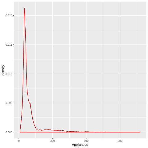
%%R
ggplot(Energy_Data, aes(x = Appliances)) + 
  geom_density(trim = TRUE) + 
  geom_density(data = Energy_Data, trim = TRUE, col = "red")

## Ensemble Exploration

#To understand how the ensemble works, let's take a peek inside the 
#Stacked Ensemble "All Models" model.  The "All Models" ensemble is 
#an ensemble of all of the individual models in the AutoML run.  
#This is often the top performing model on the leaderboard.



# Get model ids for all models in the AutoML Leaderboard
model_ids <- as.data.frame(aml@leaderboard$model_id)[,1]
# Get the "All Models" Stacked Ensemble model
se <- h2o.getModel(grep("StackedEnsemble_AllModels", model_ids, value = TRUE)[1])
# Get the Stacked Ensemble metalearner model
metalearner <- h2o.getModel(se@model$metalearner$name)

/content

auto-sklearn

auto-sklearn is an automated machine learning toolkit and a drop-in replacement for a scikit-learn estimator. It provides a scikit-learn-like interface in Python and uses Bayesian optimization to find good machine learning pipelines.

It uses automatic ensemble construction and Meta-learning to warm-start the search procedure, this means that the search is more likely to start with good pipelines. Auto-sklearn can be installed using either pip or conda commands. An example code fro training a regression model is given below

!ruby -e "$(curl -fsSL https://raw.githubusercontent.com/Homebrew/install/master/install)" < /dev/null 2> /dev/null
!brew install swig
!swig -version

!pip install swig
!pip install pyrfr
!scikit-learn
!pip install auto-sklearn

/bin/bash: brew: command not found
/bin/bash: swig: command not found

import autosklearn.classification
import sklearn.model_selection
import sklearn.datasets
import sklearn.datasets
import sklearn.metrics
import autosklearn.regression




#automl = autosklearn.classification.AutoSklearnClassifier()
#automl.fit(train_y, train_y)
#y_hat = automl.predict(test_y)
#print("Accuracy score", sklearn.metrics.accuracy_score(test_y, y_hat))

feature_types = (['numerical'] * 27))

automl = autosklearn.regression.AutoSklearnRegressor(
        time_left_for_this_task=120,
        per_run_time_limit=30,
        tmp_folder='/tmp/',
        output_folder='/tmp/',
    )
automl.fit(train_x, train_y,
               feat_type=feature_types)

print(automl.show_models())
predictions = automl.predict(test_x)
print("R2 score:", sklearn.metrics.r2_score(test_y, predictions))

Automatic Deep Learning

AutoKeras is an open source software library for automated machine learning (AutoML). The ultimate goal of AutoML is to provide easily accessible deep learning tools to domain experts with limited data science or machine learning background. AutoKeras provides functions to automatically search for architecture and hyperparameters of deep learning models. This makes very slow because it requires full retraining from scratch of each model AutoKeras is useful for (2D) Image classification. Many other ML deep learning task has not been implemented so far. Auto-Keras uses network morphism to reduce training time in neural architecture search. Further, it uses a Gaussian process (GP) for Bayesian optimization of guiding network morphism.

!!pip install autokeras

['Collecting autokeras',
 '\x1b[?25l  Downloading https://files.pythonhosted.org/packages/c2/32/de74bf6afd09925980340355a05aa6a19e7378ed91dac09e76a487bd136d/autokeras-0.4.0.tar.gz (67kB)',
 '', |

from tensorflow import keras
from keras.datasets import mnist
from autokeras.image.image_supervised import ImageClassifier

(x_train, y_train), (x_test, y_test) = mnist.load_data()
x_train = x_train.reshape(x_train.shape + (1,))
x_test = x_test.reshape(x_test.shape + (1,))

clf = ImageClassifier(verbose=True)
clf.fit(x_train, y_train, time_limit=12 * 60 * 60)
clf.final_fit(x_train, y_train, x_test, y_test, retrain=True)
y = clf.evaluate(x_test, y_test)
print(y)

/usr/local/lib/python3.6/dist-packages/tensorflow/python/framework/dtypes.py:526: FutureWarning: Passing (type, 1) or '1type' as a synonym of type is deprecated; in a future version of numpy, it will be understood as (type, (1,)) / '(1,)type'.
  _np_qint8 = np.dtype([("qint8", np.int8, 1)])
/usr/local/lib/python3.6/dist-packages/tensorflow/python/framework/dtypes.py:527: FutureWarning: Passing (type, 1) or '1type' as a synonym of type is deprecated; in a future version of numpy, it will be understood as (type, (1,)) / '(1,)type'.
  _np_quint8 = np.dtype([("quint8", np.uint8, 1)])
/usr/local/lib/python3.6/dist-packages/tensorflow/python/framework/dtypes.py:528: FutureWarning: Passing (type, 1) or '1type' as a synonym of type is deprecated; in a future version of numpy, it will be understood as (type, (1,)) / '(1,)type'.
  _np_qint16 = np.dtype([("qint16", np.int16, 1)])
/usr/local/lib/python3.6/dist-packages/tensorflow/python/framework/dtypes.py:529: FutureWarning: Passing (type, 1) or '1type' as a synonym of type is deprecated; in a future version of numpy, it will be understood as (type, (1,)) / '(1,)type'.
  _np_quint16 = np.dtype([("quint16", np.uint16, 1)])
/usr/local/lib/python3.6/dist-packages/tensorflow/python/framework/dtypes.py:530: FutureWarning: Passing (type, 1) or '1type' as a synonym of type is deprecated; in a future version of numpy, it will be understood as (type, (1,)) / '(1,)type'.
  _np_qint32 = np.dtype([("qint32", np.int32, 1)])
/usr/local/lib/python3.6/dist-packages/tensorflow/python/framework/dtypes.py:535: FutureWarning: Passing (type, 1) or '1type' as a synonym of type is deprecated; in a future version of numpy, it will be understood as (type, (1,)) / '(1,)type'.
  np_resource = np.dtype([("resource", np.ubyte, 1)])

The default version of TensorFlow in Colab will soon switch to TensorFlow 2.x.
We recommend you upgrade now or ensure your notebook will continue to use TensorFlow 1.x via the %tensorflow_version 1.x magic: more info.

Using TensorFlow backend.


Better speed can be achieved with apex installed from https://www.github.com/nvidia/apex.
Downloading data from https://s3.amazonaws.com/img-datasets/mnist.npz
11493376/11490434 [==============================] - 1s 0us/step
Saving Directory: /tmp/autokeras_NEPR81
Preprocessing the images.
Preprocessing finished.

Initializing search.
Initialization finished.


+----------------------------------------------+
|               Training model 0               |
+----------------------------------------------+
                                                                                                    
No loss decrease after 5 epochs.


Saving model.
+--------------------------------------------------------------------------+
|        Model ID        |          Loss          |      Metric Value      |
+--------------------------------------------------------------------------+
|           0            |   0.4400691822171211   |         0.9648         |
+--------------------------------------------------------------------------+


+----------------------------------------------+
|               Training model 1               |
+----------------------------------------------+

No loss decrease after 5 epochs.


Saving model.
+--------------------------------------------------------------------------+
|        Model ID        |          Loss          |      Metric Value      |
+--------------------------------------------------------------------------+
|           1            |  0.07899918230250477   |         0.9936         |
+--------------------------------------------------------------------------+


+----------------------------------------------+
|               Training model 2               |
+----------------------------------------------+
Epoch-6, Current Metric - 0.97:  77%|███████████████████▎     | 360/465 [01:57<00:35,  2.96 batch/s]

auto_ml

auto_ml is designed for production. It is very simple to use and turning out to be one of my favorites. More informattion on this package can be found here. You can train XGBoost, Deep Leaarning with TensorFlow & Keras,CatBoost and LightGBM which are all integrated with auto_ml. Generally, just pass one of them in for model_names. ml_predictor.train(data, model_names=[‘DeepLearningClassifier’]).

Available options are - DeepLearningClassifier and DeepLearningRegressor - XGBClassifier and XGBRegressor - LGBMClassifier and LGBMRegressor. Among the numerous automation this package provides include feature engineering like one-hot encoding, creating new features like day_of_week,minutes etc from date-time features, feature normalization etc.

!pip install dill
!pip install -r advanced_requirements.txt,
!pip install auto_ml
!pip install xgboost
!pip install catboost
!pip install tensorflow
!pip install keras
!pip install ipywidgets
!jupyter nbextension enable --py widgetsnbextension

Requirement already satisfied: pygments in /usr/local/lib/python3.6/dist-packages (from ipython>=4.0.0; python_version >= "3.3"->ipywidgets) (2.1.3)
Requirement already satisfied: simplegeneric>0.8 in /usr/local/lib/python3.6/dist-packages (from ipython>=4.0.0; python_version >= "3.3"->ipywidgets) (0.8.1)

from auto_ml import Predictor
from auto_ml.utils import get_boston_dataset
from auto_ml.utils_models import load_ml_model

column_descriptions = {
    'Appliances': 'output',
    #'CHAS': 'categorical'
}

train_data= pd.concat([train_x,train_y],axis=1)
ml_predictor = Predictor(type_of_estimator='regressor', 
                         column_descriptions=column_descriptions
                         )

#ml_predictor.train(train_data,model_names=['DeepLearningRegressor']), r2=0.22
#ml_predictor.train(train_data,model_names=['XGBRegressor'])  #r2=0.32
#ml_predictor.train(train_data,model_names=['LGBMRegressor']) #0.497
ml_predictor.train(train_data)   #0.431

ml_predictor.score(test_x, test_y)

Welcome to auto_ml! We're about to go through and make sense of your data using machine learning, and give you a production-ready pipeline to get predictions with.

If you have any issues, or new feature ideas, let us know at http://auto.ml
You are running on version 2.9.10
Now using the model training_params that you passed in:
{}
After overwriting our defaults with your values, here are the final params that will be used to initialize the model:
{'presort': False, 'learning_rate': 0.1, 'warm_start': True}
Running basic data cleaning
Fitting DataFrameVectorizer
Now using the model training_params that you passed in:
{}
After overwriting our defaults with your values, here are the final params that will be used to initialize the model:
{'presort': False, 'learning_rate': 0.1, 'warm_start': True}


********************************************************************************************
About to fit the pipeline for the model GradientBoostingRegressor to predict Appliances
Started at:
2019-12-16 01:53:15
[1] random_holdout_set_from_training_data's score is: -103.844
[2] random_holdout_set_from_training_data's score is: -102.638
[3] random_holdout_set_from_training_data's score is: -101.687
[4] random_holdout_set_from_training_data's score is: -100.815
[5] random_holdout_set_from_training_data's score is: -100.113
[6] random_holdout_set_from_training_data's score is: -99.56
[7] random_holdout_set_from_training_data's score is: -99.099
[8] random_holdout_set_from_training_data's score is: -98.695
[9] random_holdout_set_from_training_data's score is: -98.152
[10] random_holdout_set_from_training_data's score is: -97.829
[11] random_holdout_set_from_training_data's score is: -97.534
[12] random_holdout_set_from_training_data's score is: -97.089

 :
 :
 :
 
[9700] random_holdout_set_from_training_data's score is: -78.201
[9800] random_holdout_set_from_training_data's score is: -78.196
[9900] random_holdout_set_from_training_data's score is: -78.183
The number of estimators that were the best for this training dataset: 9200
The best score on the holdout set: -78.17831855991089
Finished training the pipeline!
Total training time:
0:19:50


Here are the results from our GradientBoostingRegressor
predicting Appliances
Calculating feature responses, for advanced analytics.


/usr/local/lib/python3.6/dist-packages/sklearn/model_selection/_split.py:2179: FutureWarning: From version 0.21, test_size will always complement train_size unless both are specified.
  FutureWarning)


The printed list will only contain at most the top 100 features.
+----+----------------+--------------+---------+-------------------+-------------------+-----------+-----------+-----------+-----------+
|    | Feature Name   |   Importance |   Delta |   FR_Decrementing |   FR_Incrementing |   FRD_abs |   FRI_abs |   FRD_MAD |   FRI_MAD |
|----+----------------+--------------+---------+-------------------+-------------------+-----------+-----------+-----------+-----------|
| 33 | year           |       0.0000 |  0.0000 |            0.0000 |            0.0000 |    0.0000 |    0.0000 |    0.0000 |    0.0000 |
| 32 | quarter        |       0.0004 |  0.2454 |            0.0000 |            0.0000 |    0.0000 |    0.0000 |    0.0000 |    0.0000 |
| 29 | month          |       0.0044 |  0.6681 |            1.8807 |           -0.5714 |    2.7292 |    0.7609 |    0.1994 |    0.0000 |
| 31 | weekday        |       0.0096 |  1.0071 |            1.1695 |           -1.1261 |    3.9296 |    4.1527 |    1.0363 |    0.9279 |
| 23 | Visibility     |       0.0121 |  5.9874 |            2.5418 |            1.7824 |    5.9795 |    4.3472 |    1.6654 |    1.6835 |
| 28 | day            |       0.0149 |  4.2629 |           -1.1345 |            8.7127 |    3.9208 |   12.0951 |    1.0589 |    1.2265 |
| 25 | rv1            |       0.0157 |  7.1657 |           56.4534 |           96.4440 |   57.2148 |   97.1504 |   47.4928 |   64.5670 |
| 26 | rv2            |       0.0178 |  7.1657 |           65.4006 |           66.8796 |   66.3326 |   67.5132 |   60.2277 |   60.9206 |
|  1 | T1             |       0.0188 |  0.7852 |           13.8211 |            1.1122 |   19.1298 |    9.2902 |    8.3319 |    3.7755 |
| 17 | T9             |       0.0204 |  0.9972 |            3.8749 |           17.1198 |   12.5666 |   23.9141 |    6.9691 |   13.0813 |
| 30 | week           |       0.0213 |  2.8238 |            6.6785 |            8.0968 |    9.4417 |   12.5097 |    3.7337 |    1.9681 |
| 22 | Windspeed      |       0.0219 |  1.2516 |            0.3866 |            2.6343 |    7.8313 |    7.5808 |    4.5071 |    2.9881 |
| 13 | T7             |       0.0229 |  1.0471 |           19.2027 |            2.7276 |   24.3899 |   11.8721 |    6.9290 |    5.4307 |
| 21 | RH_out         |       0.0230 |  7.5409 |            4.5123 |            5.7414 |   10.1780 |   10.9347 |    4.3237 |    4.2214 |
|  7 | T4             |       0.0234 |  1.0108 |            4.8105 |            3.0581 |   11.4415 |   11.6706 |    6.1204 |    5.2510 |
|  3 | T2             |       0.0235 |  1.0783 |           14.0835 |            0.8992 |   19.7000 |   11.4377 |    6.4855 |    5.7581 |
| 19 | T_out          |       0.0239 |  2.6511 |            6.8862 |           -4.4735 |   18.3031 |   10.5233 |   10.0484 |    7.6458 |
|  9 | T5             |       0.0240 |  0.9025 |           13.1377 |            3.0813 |   19.8936 |   10.4180 |    7.6748 |    4.9818 |
| 18 | RH_9           |       0.0264 |  2.0675 |            5.6641 |            0.8102 |   13.4686 |   13.8479 |    8.2520 |    8.7596 |
| 24 | Tdewpoint      |       0.0299 |  2.0609 |            2.5114 |            5.8576 |   15.2535 |   15.9113 |    7.3289 |    8.4186 |
|  0 | lights         |       0.0302 |  3.9307 |            0.0000 |            0.0000 |    0.0000 |    0.0000 |    0.0000 |    0.0000 |
| 12 | RH_6           |       0.0324 | 15.9312 |            6.9685 |           23.3361 |   14.6424 |   29.8704 |    5.8741 |    9.1803 |
| 16 | RH_8           |       0.0334 |  2.6452 |            5.3547 |            1.5003 |   18.7197 |   13.6153 |    9.8327 |    7.8713 |
| 11 | T6             |       0.0343 |  3.0657 |            0.7589 |           13.1492 |   20.2709 |   21.9876 |   11.7236 |   10.2991 |
| 14 | RH_7           |       0.0353 |  2.5387 |           12.6561 |            2.0688 |   18.6964 |   12.7747 |    8.9771 |    6.7723 |
|  8 | RH_4           |       0.0372 |  2.1545 |           14.7021 |           11.6144 |   21.2902 |   19.7052 |    7.5457 |    6.6670 |
| 15 | T8             |       0.0375 |  0.9570 |           -3.6613 |           10.3051 |   15.2607 |   14.0218 |    9.4964 |    8.0907 |
| 10 | RH_5           |       0.0381 |  4.6173 |           34.8231 |            0.3044 |   39.5146 |    8.5136 |   10.9724 |    4.7449 |
|  2 | RH_1           |       0.0390 |  1.9196 |            0.8117 |           12.8458 |   17.0123 |   18.3431 |    9.3164 |   10.8043 |
|  4 | RH_2           |       0.0426 |  1.9942 |           14.9731 |            1.1853 |   17.7433 |   15.2093 |    8.9040 |    8.3585 |
|  6 | RH_3           |       0.0441 |  1.5894 |            8.8671 |           16.8765 |   23.3520 |   19.1881 |    9.8736 |   11.1776 |
| 20 | Press_mm_hg    |       0.0484 |  3.6523 |            7.5979 |           12.3749 |   18.9428 |   23.5722 |    7.7871 |    8.6312 |
|  5 | T3             |       0.0491 |  0.9847 |           19.9205 |            5.5366 |   27.4795 |   16.7018 |   10.3640 |   10.0421 |
| 27 | hour           |       0.1439 |  3.3978 |            2.3847 |           -1.8274 |   20.2401 |   21.1750 |   11.4552 |   14.4227 |
+----+----------------+--------------+---------+-------------------+-------------------+-----------+-----------+-----------+-----------+


*******
Legend:
Importance = Feature Importance
     Explanation: A weighted measure of how much of the variance the model is able to explain is due to this column
FR_delta = Feature Response Delta Amount
     Explanation: Amount this column was incremented or decremented by to calculate the feature reponses
FR_Decrementing = Feature Response From Decrementing Values In This Column By One FR_delta
     Explanation: Represents how much the predicted output values respond to subtracting one FR_delta amount from every value in this column
FR_Incrementing = Feature Response From Incrementing Values In This Column By One FR_delta
     Explanation: Represents how much the predicted output values respond to adding one FR_delta amount to every value in this column
FRD_MAD = Feature Response From Decrementing- Median Absolute Delta
     Explanation: Takes the absolute value of all changes in predictions, then takes the median of those. Useful for seeing if decrementing this feature provokes strong changes that are both positive and negative
FRI_MAD = Feature Response From Incrementing- Median Absolute Delta
     Explanation: Takes the absolute value of all changes in predictions, then takes the median of those. Useful for seeing if incrementing this feature provokes strong changes that are both positive and negative
FRD_abs = Feature Response From Decrementing Avg Absolute Change
     Explanation: What is the average absolute change in predicted output values to subtracting one FR_delta amount to every value in this column. Useful for seeing if output is sensitive to a feature, but not in a uniformly positive or negative way
FRI_abs = Feature Response From Incrementing Avg Absolute Change
     Explanation: What is the average absolute change in predicted output values to adding one FR_delta amount to every value in this column. Useful for seeing if output is sensitive to a feature, but not in a uniformly positive or negative way
*******

None


***********************************************
Advanced scoring metrics for the trained regression model on this particular dataset:

Here is the overall RMSE for these predictions:
78.12730544452076

Here is the average of the predictions:
99.33728042751186

Here is the average actual value on this validation set:
98.55429826042898

Here is the median prediction:
71.29957584827399

Here is the median actual value:
60.0

Here is the mean absolute error:
39.930776664246636

Here is the median absolute error (robust to outliers):
17.292385522544976

Here is the explained variance:
0.43110768950362766

Here is the R-squared value:
0.4310505453591652
Count of positive differences (prediction > actual):
3353
Count of negative differences:
2568
Average positive difference:
35.947832693155526
Average negative difference:
-45.131248290052


***********************************************







-78.12730544452076

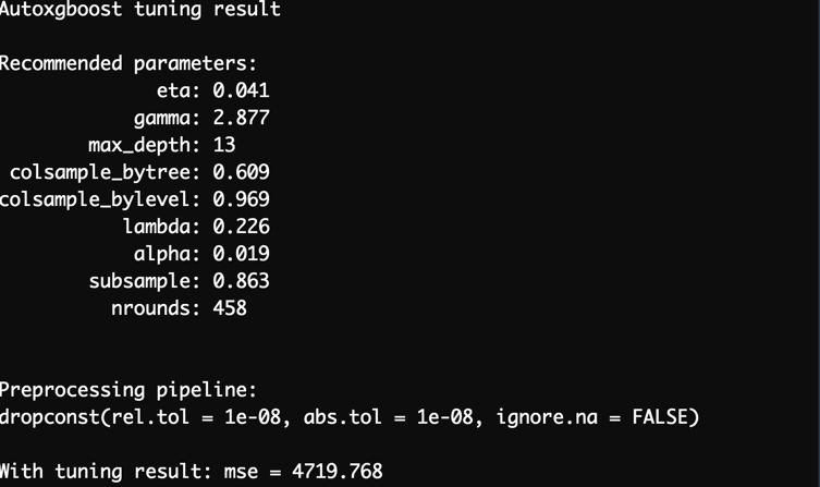
autoxgboost

source | documentation | R | Optimization: Bayesian Optimization | -

autoxgboost aims to find an optimal xgboost model automatically using the machine learning framework mlr and the bayesian optimization framework mlrMBO.

Autoxgboost is different from most frameworks on this page in that it does not search over multiple learning algorithms. Instead, it restricts itself to finding a good hyperparameter configuration for xgboost. The exception to this is a preprocessing step for categorical variables, where the specific encoding strategy to use is tuned as well.

%%R
install.packages("devtools")
install.packages("usethis")
install.packages("remotes")
install.packages("githubinstall")
install.packages("ghit")

#remotes::install_github("edwardcooper/automl")
library("devtools")
library(githubinstall)
# library("ghit")
#devtools::install_github("ja-thomas/autoxgboost")
remotes::install_github("ja-thomas/autoxgboost")
#ghit::install_github("cloudyr/ghit")
# githubinstall("autoxgboost")

%%R

library(autoxgboost)


#install.packages("devtools")
#install.packages("usethis")
#install.packages("remotes")
#remotes::install_github("edwardcooper/automl")
library("devtools")
pacman::p_load(lime,DALEX,forcats,ALEPlot,pdp,iBreakDown,localModel,breakDown,
              xfun,clipr,clipr,sf,spdep,lubrridate)
library(tidyverse)
#devtools::install_github("ja-thomas/autoxgboost")
#remotes::install_github("ja-thomas/autoxgboost")
file= '/Users/energydata_complete.csv'
energy_data= readr::read_csv(file)

energy_data$hour  = hour(energy_data$date)
energy_data$day =   wday(energy_data$date)
energy_data$month = month(energy_data$date)
energy_data$week =  week(energy_data$date)
#energy_data$weekday= weekdays(energy_data$date)
energy_data$quarter=quarter(energy_data$date)
energy_data$year =   year(energy_data$date)




energydata  =
  energy_data %>%select(-date)




library(rsample)

data_split <- initial_split(energydata, strata = "Appliances", prop = 0.70)

energydata_train <- training(data_split)
energydata_test  <- testing(data_split)

reg_task <- makeRegrTask(data = energydata_train, target = "Appliances")
set.seed(1234)
#system.time(reg_auto <- autoxgboost(reg_task))
# saveRDS(reg_auto, file = "D:/SDIautoxgboost_80.rds")


#data.task = makeRegrTask(data = iris, target = "Appliances")
ctrl = makeMBOControl()
ctrl = setMBOControlTermination(ctrl, iters = 2L) #Speed up Tuning by only doing 1 iteration
res = autoxgboost(reg_task, control = ctrl, tune.threshold = FALSE)
print(res)

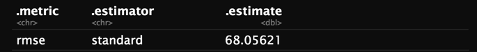
pred=predict(res,data.frame(energydata_test))

library(yardstick)pred$data


print(yardstick::rmse(pred$data,truth,response))
print(yardstick::rsq(pred$data,truth,response))

/usr/local/lib/python3.6/dist-packages/rpy2/rinterface/__init__.py:146: RRuntimeWarning: Installing package into ‘/usr/local/lib/R/site-library’
(as ‘lib’ is unspecified)

  warnings.warn(x, RRuntimeWarning)