ROC curves and AUC values are common evaluation metric for binary classification models. Although there are some criticism of it especially its’s appropritatenes in evaluating models built with imbalanced data, they still remain the most popular evaluation metric for binary classification models. In the case of highly imbalanced classification, the area under the precision- recall curve may be an appropriate evaluation metric for comparing models and measuring performance of machine learning models. There are several packages in R for evaluating the area under the ROC curve in R. The pkgsearch can be used to search for packages information on packages for performing a particular task in R including downloads last month,version,bug reports etc.
library(tidyverse) # for data manipulation
## Warning: package 'tidyverse' was built under R version 3.6.1
## Warning: package 'dplyr' was built under R version 3.6.1
library(dlstats) # for package download stats
## Warning: package 'dlstats' was built under R version 3.6.1
library(pkgsearch) # for searching packages
## Warning: package 'pkgsearch' was built under R version 3.6.1
pacman::p_load(ggthemes,scales,ggpubr,viridis,bench,microbenchmark,ggbeeswarm)

options(dplyr.width = Inf)
options(dplyr.length = Inf)
theme_set(theme_pubclean())
#methods("as.Date")


aucPkg <-  pkg_search(query="AUC",size=200,format = "short")


glimpse(aucPkg)
## Observations: 66
## Variables: 14
## $ score                <dbl> 4536.9720, 2341.1100, 2113.6843, 1979.541...
## $ package              <chr> "caTools", "AUC", "pROC", "aucm", "maxadj...
## $ version              <pckg_vrs> 1.17.1.2, 0.3.0, 1.15.3, 2018.1.24, ...
## $ title                <chr> "Tools: moving window statistics, GIF, Ba...
## $ description          <chr> "Contains several basic utility functions...
## $ date                 <dttm> 2019-03-06 19:53:35, 2013-09-30 17:41:33...
## $ maintainer_name      <chr> "ORPHANED", "Michel Ballings", "Xavier Ro...
## $ maintainer_email     <chr> "ORPHANED", "Michel.Ballings@UGent.be", "...
## $ revdeps              <int> 31, 9, 79, 2, 1, 2, 1, 1, 1, 1, 1, 1, 1, ...
## $ downloads_last_month <int> 213594, 5788, 89924, 454, 259, 835, 361, ...
## $ license              <chr> "GPL-3", "GPL (>= 2)", "GPL (>= 3)", "GPL...
## $ url                  <chr> NA, NA, "http://expasy.org/tools/pROC/", ...
## $ bugreports           <chr> NA, NA, "https://github.com/xrobin/pROC/i...
## $ package_data         <I<list>> 2019-03-...., 2013-09-...., 2019-07-....
aucPkgShort <- aucPkg %>% as_tibble(aucPkg)%>%

  filter(maintainer_name != "ORPHANED", score > 20) %>%
  select(score, package, downloads_last_month) %>%
  arrange(desc(downloads_last_month))

head(aucPkgShort)
## # A tibble: 6 x 3
##   score package         downloads_last_month
##   <dbl> <chr>                          <int>
## 1 2114. pROC                           89924
## 2  115. rattle                         15064
## 3 2341. AUC                             5788
## 4  266. varImp                          2726
## 5  470. survAUC                         2071
## 6  391. PresenceAbsence                 1740
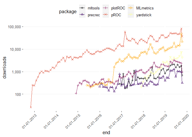
dlstats package can be used to retrieve CRAN or bioconductor package downloading statistics.
shortList <- c("mltools","precrec","plotROC","pROC","MLmetrics","yardstick")


dlstats::cran_stats(shortList) %>% group_by(package) %>% summarise(n=sum(downloads) )%>%
            arrange(desc(n))
## # A tibble: 6 x 2
##   package         n
##   <fct>       <int>
## 1 pROC      1446323
## 2 MLmetrics  364132
## 3 plotROC     62338
## 4 yardstick   56507
## 5 mltools     31904
## 6 precrec     20470
downloads <- dlstats::cran_stats(shortList) %>%

            arrange(desc(downloads))

head(downloads)
##        start        end downloads package
## 1 2019-09-01 2019-09-30     83147    pROC
## 2 2017-02-01 2017-02-28     58789    pROC
## 3 2019-03-01 2019-03-31     52335    pROC
## 4 2019-06-01 2019-06-30     50982    pROC
## 5 2019-05-01 2019-05-31     49750    pROC
## 6 2019-04-01 2019-04-30     49243    pROC
The graph below illustrates the popularity of some the common packages for finding AUC in R. The pROC looks to be the most popular. Some of these popular packages have issues such as breaking down when the input is a very large vector or the data very imbalanced, they can evaluate to different AUC values. The goal of this post is investigate which of these packages is robust and evaluates consistent AUC values. The Stack Overflow link here talks about some of these diferences between packages. fOR EXAMPLE the PRROC package computes the AUC for the random forest model trained in theis post as 0.5 wheras most of the other packages compute the AUC value as 0.984898. This snapshot shows an example where the MLmetrics package breaks down for a vector of size around 600,000.

ggplot(downloads, aes(end, downloads, group=package, color=package )) +

  geom_line() +


  geom_point(aes(shape=package)) +


  scale_y_continuous(trans = log10_trans(), labels =  scales::comma)+

  #scale_fill_viridis_d()+
  scale_color_viridis_d(option="B") +

   scale_shape_manual(values = 1:6 )  +

 #   theme_economist() +

  scale_x_date(labels = date_format("%d-%m-%Y"),date_breaks = "1 year") +
  theme(axis.text.x=element_text(angle=45, hjust=1))
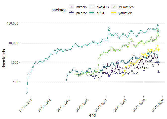
shortList <- c("mltools","precrec","plotROC","pROC","MLmetrics","yardstick")
downloads <- dlstats::bioc_stats(shortList)
head(downloads)
##        start        end downloads package
## 1 2016-11-01 2016-11-30       285 mltools
## 2 2016-12-01 2016-12-31       272 mltools
## 3 2017-01-01 2017-01-31       793 mltools
## 4 2017-02-01 2017-02-28       179 mltools
## 5 2017-03-01 2017-03-31       190 mltools
## 6 2017-04-01 2017-04-30       382 mltools
ggplot(downloads, aes(end, downloads, group=package, color=package )) +

  geom_line() +


  geom_point(aes(shape=package)) +


  scale_y_continuous(trans = log10_trans(), labels =  scales::comma)+

  #scale_fill_viridis_d()+
  scale_color_viridis_d(option="D") +

   scale_shape_manual(values = 1:9 )  +

 #   theme_economist() +

  scale_x_date(labels = date_format("%d-%m-%Y"),date_breaks = "1 year") +
  theme(axis.text.x=element_text(angle=45, hjust=1))
Train Random Forest Model
library(randomForest) # basic implementation
library(ranger)
#install packages
#install.packages("ROSE")
library(ROSE)
## Warning: package 'ROSE' was built under R version 3.6.1
data(hacide)
glimpse(hacide.train)
## Observations: 1,000
## Variables: 3
## $ cls <fct> 0, 0, 0, 0, 0, 0, 0, 0, 0, 0, 0, 0, 0, 0, 0, 0, 0, 0, 0, 0...
## $ x1  <dbl> 0.20079810, 0.01662009, 0.22872469, 0.12637877, 0.60082129...
## $ x2  <dbl> 0.67803761, 1.57655790, -0.55953375, -0.09381378, -0.29839...
table(hacide.train$cls)
##
##   0   1
## 980  20
#check classes distribution
prop.table(table(hacide.train$cls))
##
##    0    1
## 0.98 0.02
data.rose <- ROSE(cls ~ ., data = hacide.train, seed = 1)$data
table(data.rose$cls)
##
##   0   1
## 520 480
#build a random forest models

m1 <- randomForest(
  formula = cls ~ .,
  data    = data.rose
)

#make predictions on unseen data
pred.prob <- predict(m1, newdata = hacide.test,type = "prob")


pred.class <- predict(m1, newdata = hacide.test)


ROSE::roc.curve(hacide.test$cls,pred.prob[,2])
## Area under the curve (AUC): 0.985
AUC function
ROC_AUC <- function(y_predprob, y_true) {


  #sum of positive labels
    n_pos <- sum(y_true)
  #sum of negative labels
  n_neg = sum(y_true==0)
  A  <- sum(rank(y_predprob)[!y_true]) - n_neg * (n_neg + 1) / 2
  return(1 - A /( n_neg*  n_pos)  )
}


ROC_AUC(pred.prob[,2],as.double(hacide.test$cls)-1)
## [1] 0.984898
MLmetrics
MLmetrics::AUC(pred.prob[,2],hacide.test$cls)
## [1] 0.984898
pROC
library(pROC)
## Warning: package 'pROC' was built under R version 3.6.1
## Type 'citation("pROC")' for a citation.
##
## Attaching package: 'pROC'
## The following objects are masked from 'package:stats':
##
##     cov, smooth, var
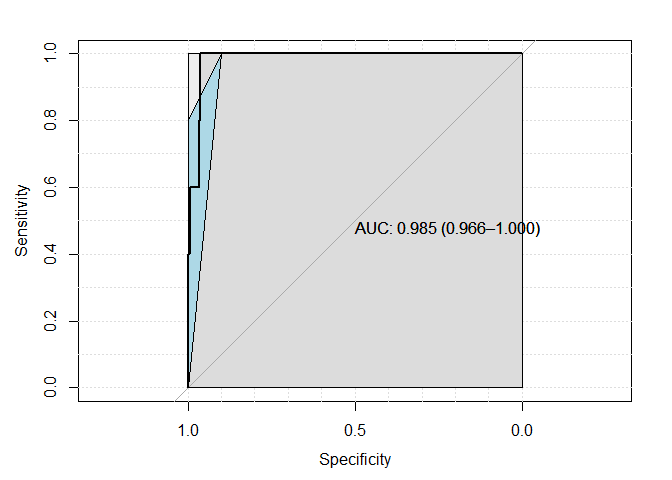
pROC_obj <- roc(hacide.test$cls,pred.prob[,2],
                smoothed = TRUE,
                # arguments for ci
                ci=TRUE, ci.alpha=0.9, stratified=FALSE,
                # arguments for plot
                plot=TRUE, auc.polygon=TRUE, max.auc.polygon=TRUE, grid=TRUE,
                print.auc=TRUE, show.thres=TRUE)
## Setting levels: control = 0, case = 1
## Setting direction: controls < cases
sens.ci <- ci.se(pROC_obj)
plot(sens.ci, type="shape", col="lightblue")
## Warning in plot.ci.se(sens.ci, type = "shape", col = "lightblue"): Low
## definition shape.
#plot(sens.ci, type="bars")


pROC_obj <- roc(hacide.test$cls,pred.prob[,2])
## Setting levels: control = 0, case = 1
## Setting direction: controls < cases
pROC::auc(pROC_obj )
## Area under the curve: 0.9849
plotROC
library(plotROC)
## Warning: package 'plotROC' was built under R version 3.6.1
##
## Attaching package: 'plotROC'
## The following object is masked from 'package:pROC':
##
##     ggroc
df= tibble(labels=as.double(hacide.test$cls)-1,predictions=pred.prob[,2])%>%
       mutate()


rocplot <- ggplot(df, aes(m = predictions, d = labels))+ geom_roc(n.cuts=20,labels=FALSE)
rocplot + style_roc(theme = theme_grey) + geom_rocci(fill="pink")
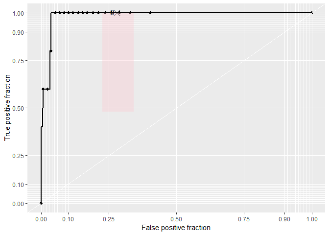
plotROC::calc_auc(rocplot)
##   PANEL group      AUC
## 1     1    -1 0.984898
precrec
library(precrec)
## Warning: package 'precrec' was built under R version 3.6.1
##
## Attaching package: 'precrec'
## The following object is masked from 'package:pROC':
##
##     auc
precrec_obj <- evalmod(scores = df$predictions, labels = df$labels)
autoplot(precrec_obj)
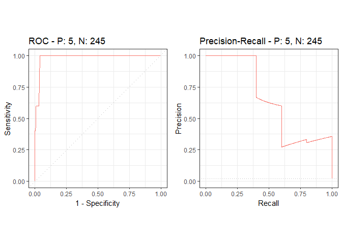
precrec::auc(precrec_obj)
##   modnames dsids curvetypes      aucs
## 1       m1     1        ROC 0.9848980
## 2       m1     1        PRC 0.6529288
mltools
library(mltools)
## Warning: package 'mltools' was built under R version 3.6.1
##
## Attaching package: 'mltools'
## The following object is masked from 'package:tidyr':
##
##     replace_na
auc_roc(df$predictions,df$labels) # 0.875
## [1] 0.984898
auc_roc(df$predictions,df$labels, returnDT=TRUE)%>%head()
##     Pred CountFalse CountTrue CumulativeFPR CumulativeTPR AdditionalArea
## 1: 1.000          0         1   0.000000000           0.2    0.000000000
## 2: 0.998          0         1   0.000000000           0.4    0.000000000
## 3: 0.974          1         0   0.004081633           0.4    0.001632653
## 4: 0.970          1         1   0.008163265           0.6    0.002040816
## 5: 0.920          1         0   0.012244898           0.6    0.002448980
## 6: 0.914          1         0   0.016326531           0.6    0.002448980
##    CumulativeArea
## 1:    0.000000000
## 2:    0.000000000
## 3:    0.001632653
## 4:    0.003673469
## 5:    0.006122449
## 6:    0.008571429
yardstick
df2=  df %>% mutate(labels= as_factor(labels))
yardstick::roc_auc(df2,labels,predictions)
## Setting direction: controls > cases
## # A tibble: 1 x 3
##   .metric .estimator .estimate
##   <chr>   <chr>          <dbl>
## 1 roc_auc binary         0.985
PRROC
library(PRROC)
## Warning: package 'PRROC' was built under R version 3.6.1
##
## Attaching package: 'PRROC'
## The following object is masked from 'package:ROSE':
##
##     roc.curve
preds_pos <- pred.prob[hacide.test$cls==1] #preds for true positive class
preds_neg <- pred.prob[hacide.test$cls==0] #preds for true negative class
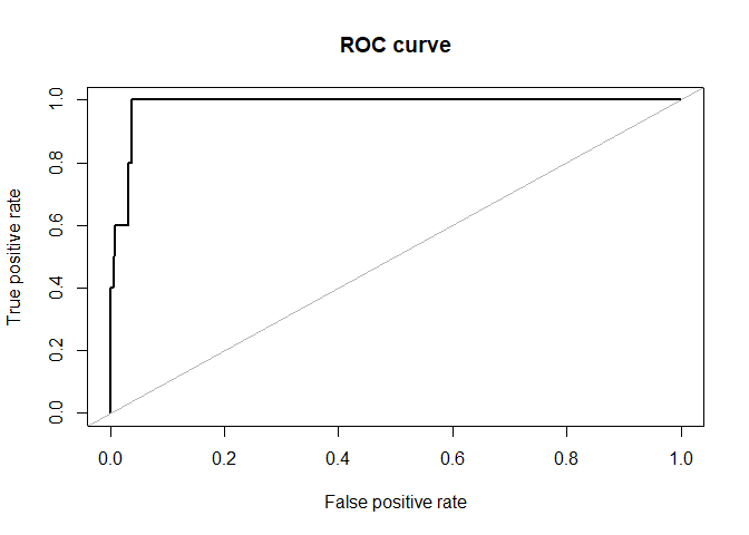
plot(PRROC::roc.curve(preds_pos, preds_neg, curve = TRUE))
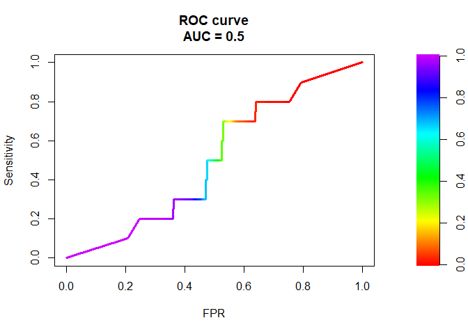
PRROC::roc.curve(preds_pos, preds_neg,curve=FALSE)
##
##   ROC curve
##
##     Area under curve:
##      0.5
##
##     Curve not computed ( can be done by using curve=TRUE )
comparing performance
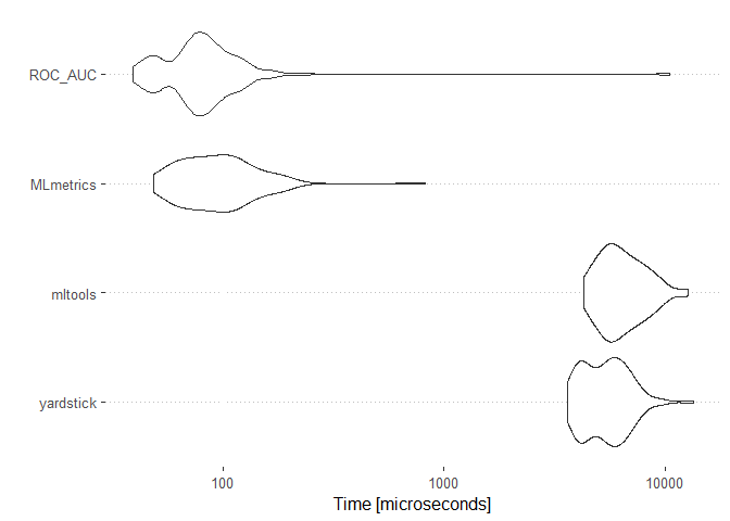
bnch <- microbenchmark(
  yardstick=yardstick::roc_auc(df2,labels,predictions)$.estimate,
  mltools= mltools::auc_roc(df$predictions,df$labels),
  MLmetrics= MLmetrics::AUC(df$predictions,df$labels),
  ROC_AUC=ROC_AUC(df$predictions,df$labels)

)
bnch
## Unit: microseconds
##       expr      min        lq      mean    median        uq      max neval
##  yardstick 3631.784 4336.6365 5541.4402 5419.5160 6376.5280 13409.27   100
##    mltools 4301.650 5373.6500 6596.2318 6176.2085 7555.8345 12705.70   100
##  MLmetrics   48.640   69.7605  106.0827   91.9475  119.4670   823.04   100
##    ROC_AUC   39.254   65.7075  187.2773   79.3605   95.3605 10513.49   100
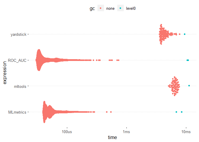
ggplot2::autoplot(bnch)
## Coordinate system already present. Adding new coordinate system, which will replace the existing one.
results <- bench::mark(
   yardstick=yardstick::roc_auc(df2,labels,predictions)$.estimate,
  mltools= mltools::auc_roc(df$predictions,df$labels),
  MLmetrics= MLmetrics::AUC(df$predictions,df$labels),
  ROC_AUC=ROC_AUC(df$predictions,df$labels)
)
as_tibble(results)
## # A tibble: 4 x 13
##   expression      min   median `itr/sec` mem_alloc `gc/sec` n_itr  n_gc
##   <bch:expr> <bch:tm> <bch:tm>     <dbl> <bch:byt>    <dbl> <int> <dbl>
## 1 yardstick    3.58ms   4.12ms      229.   140.6KB     2.03   113     1
## 2 mltools      5.07ms   6.45ms      154.   241.3KB     2.03    76     1
## 3 MLmetrics   39.25us  49.07us    18224.    14.3KB     4.16  8766     2
## 4 ROC_AUC     30.29us  36.69us    21905.    16.2KB     4.38  9998     2
##   total_time result    memory             time     gc
##     <bch:tm> <list>    <list>             <list>   <list>
## 1      493ms <dbl [1]> <df[,3] [156 x 3]> <bch:tm> <tibble [114 x 3]>
## 2      492ms <dbl [1]> <df[,3] [66 x 3]>  <bch:tm> <tibble [77 x 3]>
## 3      481ms <dbl [1]> <df[,3] [12 x 3]>  <bch:tm> <tibble [8,768 x 3]>
## 4      456ms <dbl [1]> <df[,3] [13 x 3]>  <bch:tm> <tibble [10,000 x 3]>
#summary(results, relative = TRUE)

ggplot2::autoplot(results)
library(tidyverse)
results %>%
  unnest() %>%
  filter(gc == "none") %>%
  ggplot(aes(x = mem_alloc, y = time, color = expression)) +
    geom_point() +
    scale_color_brewer(type = "qual", palette = 3) +
    geom_smooth(method = "lm", se = F, colour = "grey50")
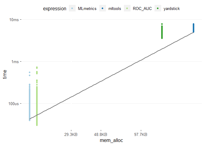
The MLmetrics package and the ROC_AUC function appears to be much faster than the other packages. On the otherhand the mltools package did not experience any break down during its usage unlike the MLmetric package.