Introduction
The two main packages in R for machine learning interpretability is the iml and DALEX. H2o package also has built in functions to perform some interpretability such as partial dependence plots. DALEX and iml are model agnostic as such can be used to explain several supervised machine learning models including xgboost,random forest, support vector machines, deep learning(keras and h2o MLP).The shapper library Implements a wrapper for the Python shap library that provides SHapley Additive exPlanations (SHAP).
Before we proceed, there are a few preprocessing steps that is used to load data from a python evironment which is then converted to an R dataframe using rpy2 package and magic functions. This post follows an earlier post on machine learning interpretability in python.
# activate R magic
import rpy2
%load_ext rpy2.ipython
#%%capture  #hide cell output
%%R
install.packages("pacman")
import numpy as np
import pandas as pd
from google.colab import files
import io
Loading Data
link to data This database contains 76 attributes, but all published experiments refer to using a subset of 14 of them. In particular, the Cleveland database is the only one that has been used by ML researchers to this date. The “goal” field refers to the presence of heart disease in the patient. It is integer valued from 0 (no presence) to 4.
Content
Attribute Information: Only 14 attributes used:
- age: age in years
- sex: sex (1 = male; 0 = female)
- cp: chest pain type – Value 1: typical angina – Value 2: atypical angina – Value 3: non-anginal pain – Value 4: asymptomatic
- trestbps: resting blood pressure (in mm Hg on admission to the hospital)
- chol: serum cholestoral in mg/dl
- fbs: (fasting blood sugar > 120 mg/dl) (1 = true; 0 = false)
- restecg: resting electrocardiographic results – Value 0: normal – Value 1: having ST-T wave abnormality (T wave inversions and/or ST elevation or depression of > 0.05 mV) – Value 2: showing probable or definite left ventricular hypertrophy by Estes’ criteria
- thalach: maximum heart rate achieved
- exang: exercise induced angina (1 = yes; 0 = no)
- oldpeak = ST depression induced by exercise relative to rest
- slope: the slope of the peak exercise ST segment – Value 1: upsloping – Value 2: flat – Value 3: downsloping
- ca: number of major vessels (0-3) colored by flourosopy
- thal: 3 = normal; 6 = fixed defect; 7 = reversable defect
- target: diagnosis of heart disease (angiographic disease status) – Value 0: < 50% diameter narrowing – Value 1: > 50% diameter narrowing (in any major vessel: attributes 59 through 68 are vessels)
#uploaded = files.upload()
#for fn in uploaded.keys():
#  print('User uploaded file "{name}" with length {length} bytes'.format(
#      name=fn, length=len(uploaded[fn])))
heart_data=pd.read_csv('https://raw.githubusercontent.com/NanaAkwasiAbayieBoateng/Datasets/master/heart.csv')
heart_data.head()
| age | sex | cp | trestbps | chol | fbs | restecg | thalach | exang | oldpeak | slope | ca | thal | target | |
|---|---|---|---|---|---|---|---|---|---|---|---|---|---|---|
| 0 | 63 | 1 | 3 | 145 | 233 | 1 | 0 | 150 | 0 | 2.3 | 0 | 0 | 1 | 1 |
| 1 | 37 | 1 | 2 | 130 | 250 | 0 | 1 | 187 | 0 | 3.5 | 0 | 0 | 2 | 1 |
| 2 | 41 | 0 | 1 | 130 | 204 | 0 | 0 | 172 | 0 | 1.4 | 2 | 0 | 2 | 1 |
| 3 | 56 | 1 | 1 | 120 | 236 | 0 | 1 | 178 | 0 | 0.8 | 2 | 0 | 2 | 1 |
| 4 | 57 | 0 | 0 | 120 | 354 | 0 | 1 | 163 | 1 | 0.6 | 2 | 0 | 2 | 1 |
#heart_data=pd.read_csv(io.StringIO(uploaded['heart.csv'].decode('utf-8')))
#heart_data.head()
Load Required Packages
The pacman package provides a convenient way to load packages. It installs the package before loading if it not already installed.One of my favorite themes that I use with ggplot is the theme_pubclean. Here I set all themes with ggplot by it.
%%capture
%%R
pacman::p_load(tidyverse,h2o,iml,Hmisc)

pacman::p_load(tidyverse,reticulate,DataExplorer,skimr,ggpubr,viridis,
               kableExtra,caret,recipes,rsample,yardstick,pROC,
               xgboost,mlr,readxl,stringr,VIM,
               MLmetrics,data.table,furrr,ALEPlot,pdp,iBreakDown)


#Load  variable importance plot
source("https://raw.githubusercontent.com/NanaAkwasiAbayieBoateng/MLTools/master/Varplot.R")

source("https://raw.githubusercontent.com/NanaAkwasiAbayieBoateng/MLTools/master/EvaluationMetrics.R")


theme_set(theme_pubclean())
%%capture
%%R
if (!require("forcats")) {
    install.packages("forcats")
}

pacman::p_load(lime,DALEX,forcats,ALEPlot,pdp,iBreakDown,localModel,breakDown,
              xfun,clipr,clipr,sf,spdep)
# dependencies

#devtools::install_github("pbiecek/breakDown")

# DALEX package
#devtools::install_github("pbiecek/DALEX")
#devtools::install_github("MI2DataLab/factorMerger")

#install.packages("factorMerger")
#install.packages(c("devtools","DALEX","units"))
pacman::p_load(agricolae,factorMerger)
pacman::p_load(units)
#devtools::install_github("ModelOriented/shapper")

#pacman::p_load("clipr","ggplot2","rlang","xfun","agricolae","clipr","sf","spdep","breakDown",localModel)
Start h2o cluster here!
%%R
localH2O = h2o.init()
h2o.no_progress()
H2O is not running yet, starting it now...

Note:  In case of errors look at the following log files:
    /tmp/RtmpjwF5L0/h2o_UnknownUser_started_from_r.out
    /tmp/RtmpjwF5L0/h2o_UnknownUser_started_from_r.err


Starting H2O JVM and connecting: .. Connection successful!

R is connected to the H2O cluster:
    H2O cluster uptime:         2 seconds 389 milliseconds
    H2O cluster timezone:       Etc/UTC
    H2O data parsing timezone:  UTC
    H2O cluster version:        3.24.0.5
    H2O cluster version age:    11 days
    H2O cluster name:           H2O_started_from_R_root_wlr900
    H2O cluster total nodes:    1
    H2O cluster total memory:   2.94 GB
    H2O cluster total cores:    2
    H2O cluster allowed cores:  2
    H2O cluster healthy:        TRUE
    H2O Connection ip:          localhost
    H2O Connection port:        54321
    H2O Connection proxy:       NA
    H2O Internal Security:      FALSE
    H2O API Extensions:         Amazon S3, XGBoost, Algos, AutoML, Core V3, Core V4
    R Version:                  R version 3.6.0 (2019-04-26)
from rpy2.robjects import pandas2ri
pandas2ri.activate()
Rheart_data = pandas2ri.py2ri(heart_data)
type(Rheart_data)
rpy2.robjects.vectors.DataFrame
Convert Python Dataframe to R dataframe
The python dataframe can be converted to an R dataframe.
%%R -i heart_data

head(heart_data,5)
/usr/local/lib/python3.6/dist-packages/rpy2/robjects/pandas2ri.py:191: FutureWarning: from_items is deprecated. Please use DataFrame.from_dict(dict(items), ...) instead. DataFrame.from_dict(OrderedDict(items)) may be used to preserve the key order.
  res = PandasDataFrame.from_items(items)


  age sex cp trestbps chol fbs restecg thalach exang oldpeak slope ca thal
0  63   1  3      145  233   1       0     150     0     2.3     0  0    1
1  37   1  2      130  250   0       1     187     0     3.5     0  0    2
2  41   0  1      130  204   0       0     172     0     1.4     2  0    2
3  56   1  1      120  236   0       1     178     0     0.8     2  0    2
4  57   0  0      120  354   0       1     163     1     0.6     2  0    2
  target
0      1
1      1
2      1
3      1
4      1
%%R
str(heart_data)

glimpse(heart_data)
'data.frame':	303 obs. of  14 variables:
 $ age     : int  63 37 41 56 57 57 56 44 52 57 ...
 $ sex     : int  1 1 0 1 0 1 0 1 1 1 ...
 $ cp      : int  3 2 1 1 0 0 1 1 2 2 ...
 $ trestbps: int  145 130 130 120 120 140 140 120 172 150 ...
 $ chol    : int  233 250 204 236 354 192 294 263 199 168 ...
 $ fbs     : int  1 0 0 0 0 0 0 0 1 0 ...
 $ restecg : int  0 1 0 1 1 1 0 1 1 1 ...
 $ thalach : int  150 187 172 178 163 148 153 173 162 174 ...
 $ exang   : int  0 0 0 0 1 0 0 0 0 0 ...
 $ oldpeak : num  2.3 3.5 1.4 0.8 0.6 0.4 1.3 0 0.5 1.6 ...
 $ slope   : int  0 0 2 2 2 1 1 2 2 2 ...
 $ ca      : int  0 0 0 0 0 0 0 0 0 0 ...
 $ thal    : int  1 2 2 2 2 1 2 3 3 2 ...
 $ target  : int  1 1 1 1 1 1 1 1 1 1 ...
Observations: 303
Variables: 14
$ age      <int> 63, 37, 41, 56, 57, 57, 56, 44, 52, 57, 54, 48, 49, 64, 58, …
$ sex      <int> 1, 1, 0, 1, 0, 1, 0, 1, 1, 1, 1, 0, 1, 1, 0, 0, 0, 0, 1, 0, …
$ cp       <int> 3, 2, 1, 1, 0, 0, 1, 1, 2, 2, 0, 2, 1, 3, 3, 2, 2, 3, 0, 3, …
$ trestbps <int> 145, 130, 130, 120, 120, 140, 140, 120, 172, 150, 140, 130, …
$ chol     <int> 233, 250, 204, 236, 354, 192, 294, 263, 199, 168, 239, 275, …
$ fbs      <int> 1, 0, 0, 0, 0, 0, 0, 0, 1, 0, 0, 0, 0, 0, 1, 0, 0, 0, 0, 0, …
$ restecg  <int> 0, 1, 0, 1, 1, 1, 0, 1, 1, 1, 1, 1, 1, 0, 0, 1, 1, 1, 1, 1, …
$ thalach  <int> 150, 187, 172, 178, 163, 148, 153, 173, 162, 174, 160, 139, …
$ exang    <int> 0, 0, 0, 0, 1, 0, 0, 0, 0, 0, 0, 0, 0, 1, 0, 0, 0, 0, 0, 0, …
$ oldpeak  <dbl> 2.3, 3.5, 1.4, 0.8, 0.6, 0.4, 1.3, 0.0, 0.5, 1.6, 1.2, 0.2, …
$ slope    <int> 0, 0, 2, 2, 2, 1, 1, 2, 2, 2, 2, 2, 2, 1, 2, 1, 2, 0, 2, 2, …
$ ca       <int> 0, 0, 0, 0, 0, 0, 0, 0, 0, 0, 0, 0, 0, 0, 0, 0, 0, 0, 0, 2, …
$ thal     <int> 1, 2, 2, 2, 2, 1, 2, 3, 3, 2, 2, 2, 2, 2, 2, 2, 2, 2, 2, 2, …
$ target   <int> 1, 1, 1, 1, 1, 1, 1, 1, 1, 1, 1, 1, 1, 1, 1, 1, 1, 1, 1, 1, …
%%R
summarizeColumns(heart_data)
       name    type na        mean       disp median      mad min   max nlevs
1       age integer  0  54.3663366  9.0821010   55.0 10.37820  29  77.0     0
2       sex integer  0   0.6831683  0.4660108    1.0  0.00000   0   1.0     0
3        cp integer  0   0.9669967  1.0320525    1.0  1.48260   0   3.0     0
4  trestbps integer  0 131.6237624 17.5381428  130.0 14.82600  94 200.0     0
5      chol integer  0 246.2640264 51.8307510  240.0 47.44320 126 564.0     0
6       fbs integer  0   0.1485149  0.3561979    0.0  0.00000   0   1.0     0
7   restecg integer  0   0.5280528  0.5258596    1.0  0.00000   0   2.0     0
8   thalach integer  0 149.6468647 22.9051611  153.0 22.23900  71 202.0     0
9     exang integer  0   0.3267327  0.4697945    0.0  0.00000   0   1.0     0
10  oldpeak numeric  0   1.0396040  1.1610750    0.8  1.18608   0   6.2     0
11    slope integer  0   1.3993399  0.6162261    1.0  1.48260   0   2.0     0
12       ca integer  0   0.7293729  1.0226064    0.0  0.00000   0   4.0     0
13     thal integer  0   2.3135314  0.6122765    2.0  0.00000   0   3.0     0
14   target integer  0   0.5445545  0.4988348    1.0  0.00000   0   1.0     0
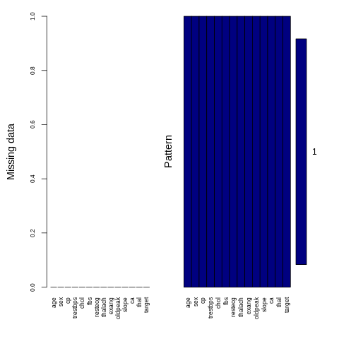
There are no issues with missing data. The data is complete.
%%R
aggr(heart_data , col=c('navyblue','yellow'),
                    numbers=TRUE, sortVars=TRUE,
                    labels=names(heart_data), cex.axis=.7,
                    gap=3, ylab=c("Missing data","Pattern"))
 Variables sorted by number of missings:
 Variable Count
      age     0
      sex     0
       cp     0
 trestbps     0
     chol     0
      fbs     0
  restecg     0
  thalach     0
    exang     0
  oldpeak     0
    slope     0
       ca     0
     thal     0
   target     0
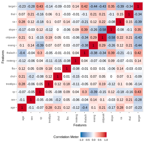
The variable thalach has moderate correlation with the age variable. There are no significant correlations between the other variables.
%%R
plot_correlation(heart_data,type = "continuous",theme_config = list(legend.position = "bottom", axis.text.x =
  element_text(angle = 90)))
Another way to obatin the summary statistics for each variable in the data is with the skim_to_wide function from the sikmr package.
%%R

skimmed <-skim_to_wide(heart_data)
skimmed
  #kable()
 # kable_styling()
# A tibble: 14 x 13
   type  variable missing complete n     mean  sd    p0    p25   p50   p75
   <chr> <chr>    <chr>   <chr>    <chr> <chr> <chr> <chr> <chr> <chr> <chr>
 1 inte… age      0       303      303   " 54… " 9.… 29    " 47… 55    " 61…
 2 inte… ca       0       303      303   "  0… " 1.… 0     "  0… 0     "  1…
 3 inte… chol     0       303      303   246.… 51.83 126   "211… 240   274.5
 4 inte… cp       0       303      303   "  0… " 1.… 0     "  0… 1     "  2…
 5 inte… exang    0       303      303   "  0… " 0.… 0     "  0… 0     "  1…
 6 inte… fbs      0       303      303   "  0… " 0.… 0     "  0… 0     "  0…
 7 inte… restecg  0       303      303   "  0… " 0.… 0     "  0… 1     "  1…
 8 inte… sex      0       303      303   "  0… " 0.… 0     "  0… 1     "  1…
 9 inte… slope    0       303      303   "  1… " 0.… 0     "  1… 1     "  2…
10 inte… target   0       303      303   "  0… " 0.… 0     "  0… 1     "  1…
11 inte… thal     0       303      303   "  2… " 0.… 0     "  2… 2     "  3…
12 inte… thalach  0       303      303   149.… 22.91 71    133.5 153   "166…
13 inte… trestbps 0       303      303   131.… 17.54 94    "120… 130   "140…
14 nume… oldpeak  0       303      303   1.04  1.16  0     0     0.8   1.6
# … with 2 more variables: p100 <chr>, hist <chr>
%%R

heart_data%>%mutate(target=as_factor(target))%>%group_by(target)%>%
summarise(n=n())%>%
    ggplot(aes(y= n,x=reorder(target,n),fill=target))+

geom_bar(stat="identity",position = position_dodge(width = 0.8),width = 0.4)+

  scale_fill_viridis(discrete = T, option = "D")+
   theme(
    # no legend
    #legend.position="none",
    plot.caption=element_text(hjust=0,size = 8),
    legend.direction="horizontal",

    legend.title = element_blank(),
    text=element_text(size=20,  family="Comic Sans MS"),

    legend.text = element_text(size = 20),# legend title size

    plot.title = element_text(hjust = 0.5,size = 16), #position legend in the middle
    plot.subtitle = element_text(hjust = 0.5,colour = "red",size = 12),
    axis.text.x = element_text(angle = 45, hjust = 1,size = 15),
    axis.text.y = element_text(size = 20))+
  labs(x="Heart Disease(yes=1,No=0)",y="Count",
       title=" ",
         subtitle=paste0(""),
         caption="" )+

  #theme(aspect.ratio = 0.2/0.1)+

geom_text(aes(label=round(n,2),vjust=-0.2),color="black",size = 6)+
  scale_y_continuous(labels = scales::number)
    #geom_text(aes(label=c(1,2),vjust=0.1),position = position_dodge(width = 1),color="black",size=5)
#glue(" RMSE: {round(rmse_val_gbm, digits = 2)}")
%%R
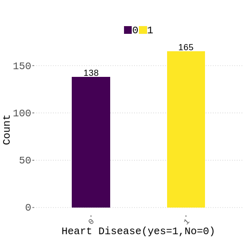
#check classes distribution
prop.table(table(heart_data$target))*100
       0        1
45.54455 54.45545
Model Building
The rsample package can be used to split the data into training and test set. Two models will be built , the elastic net logistic regression and Automatic machine learning. These models will be interpretated afterwards. Our goal is to predict predict the probability of developing a heart disease based on features such as age, sex ,cholesterol levels etc.
%%R

library(rsample)


var<-Hmisc::Cs(target, sex,cp,fbs,restecg,exang,slope,thal,ca)


heart_data<-heart_data%>%mutate_at(var, as_factor)


data_split <- initial_split(heart_data, strata = "target", prop = 0.75)

heartdata_train <- training(data_split)
heartdata_test  <- testing(data_split)
%%R

heartdata_recipe <- recipe(target ~ ., data = heartdata_train ) %>%
  #Transform numeric skewed predictors
  #step_YeoJohnson(all_numeric()) %>%
  # standardize the data
  #step_center(all_numeric(), -all_outcomes()) %>%
  #scale the data
  #step_scale(all_numeric(), -all_outcomes()) %>%
  #step_kpca a specification of a recipe step that will convert numeric data into one or more principal components using a kernel basis expansion.
  #step_kpca(all_numeric(), num=6)%>%
  #step_log(Label, base = 10)
  # Lump factor levels that occur in <= 10% of data as "other"
  #step_other(Factor_E , Factor_C , threshold = 0.1) %>%
  # Create dummy variables for all nominal predictor factor variables except the response
  #step_dummy(all_nominal(), -all_outcomes())%>%
  prep(data = heartdata_train,retain = TRUE )

# split data into training and test set
test_tbl  <- bake(heartdata_recipe, newdata = heartdata_test)
train_tbl <- bake(heartdata_recipe, newdata = heartdata_train)
glimpse(test_tbl)
Observations: 75
Variables: 14
$ age      <int> 57, 57, 44, 52, 58, 66, 43, 44, 65, 48, 53, 39, 44, 51, 34, …
$ sex      <fct> 0, 1, 1, 1, 0, 0, 1, 1, 0, 1, 0, 1, 1, 0, 1, 1, 1, 0, 1, 1, …
$ cp       <fct> 0, 0, 1, 2, 3, 3, 0, 2, 2, 1, 0, 2, 2, 2, 3, 3, 2, 1, 2, 2, …
$ trestbps <int> 120, 140, 120, 172, 150, 150, 150, 130, 155, 130, 130, 140, …
$ chol     <int> 354, 192, 263, 199, 283, 226, 247, 233, 269, 245, 264, 321, …
$ fbs      <fct> 0, 0, 0, 1, 1, 0, 0, 0, 0, 0, 0, 0, 0, 0, 0, 0, 0, 0, 0, 1, …
$ restecg  <fct> 1, 1, 1, 1, 0, 1, 1, 1, 1, 0, 0, 0, 0, 0, 0, 0, 1, 0, 1, 0, …
$ thalach  <int> 163, 148, 173, 162, 162, 114, 171, 179, 148, 180, 143, 182, …
$ exang    <fct> 1, 0, 0, 0, 0, 0, 0, 1, 0, 0, 0, 0, 0, 0, 0, 0, 1, 0, 1, 0, …
$ oldpeak  <dbl> 0.6, 0.4, 0.0, 0.5, 1.0, 2.6, 1.5, 0.4, 0.8, 0.2, 0.4, 0.0, …
$ slope    <fct> 2, 1, 2, 2, 2, 0, 2, 2, 2, 1, 1, 2, 2, 2, 2, 1, 1, 1, 2, 1, …
$ ca       <fct> 0, 0, 0, 0, 0, 0, 0, 0, 0, 0, 0, 0, 0, 0, 0, 0, 0, 0, 1, 0, …
$ thal     <fct> 2, 1, 3, 3, 2, 2, 2, 2, 2, 2, 2, 2, 2, 2, 2, 1, 2, 2, 3, 2, …
$ target   <fct> 1, 1, 1, 1, 1, 1, 1, 1, 1, 1, 1, 1, 1, 1, 1, 1, 1, 1, 1, 1, …
%%R

test=as.h2o(test_tbl)

train=as.h2o(train_tbl)


outcome_name <- "target" #response column: digits 0-1
features <- setdiff(colnames(train), outcome_name)


# try using the `categorical_encoding` parameter:
#encoding = "OneHotExplicit"
Autimatic machine learning. h2o has built in functions to handle categorical variables.
%%R

model_h2o_automl <- h2o.automl(x = features, y = outcome_name,
                  training_frame = train,
                  leaderboard_frame = test,
                  #categorical_encoding = encoding,
                  #max_models = 10,
                  max_runtime_secs = 360)
Elastic net logistic regression
%%R
# elastic net model
model_h2o_glm <- h2o.glm(
  x = features,
  y = outcome_name,
  training_frame = train,
  #categorical_encoding = encoding,
  #validation_frame = splits$valid,
  family = "binomial",
  seed = 123
  )
Gradient boosting machines
%%R
# elastic net model
model_h2o_gbm <- h2o.gbm(
  x = features,
  y = outcome_name,
  training_frame = train,
  seed = 123
  )
We can see the performance of the varoius models trained by AutoML as below.
%%R

model_h2o_automl@leaderboard%>%as_tibble()
# A tibble: 67 x 6
   model_id                          auc logloss mean_per_class_er…  rmse    mse
   <chr>                           <dbl>   <dbl>              <dbl> <dbl>  <dbl>
 1 XGBoost_grid_1_AutoML_20190630… 0.954   0.292             0.0954 0.294 0.0864
 2 GBM_4_AutoML_20190630_154827    0.953   0.306             0.113  0.303 0.0916
 3 XGBoost_3_AutoML_20190630_1548… 0.953   0.326             0.0954 0.308 0.0951
 4 XGBoost_grid_1_AutoML_20190630… 0.950   0.311             0.110  0.304 0.0926
 5 XGBoost_grid_1_AutoML_20190630… 0.949   0.303             0.115  0.299 0.0895
 6 XGBoost_grid_1_AutoML_20190630… 0.948   0.312             0.110  0.306 0.0936
 7 GBM_grid_1_AutoML_20190630_154… 0.948   0.289             0.0832 0.287 0.0825
 8 GBM_grid_1_AutoML_20190630_154… 0.948   0.598             0.105  0.363 0.132
 9 GBM_grid_1_AutoML_20190630_154… 0.947   0.334             0.0954 0.315 0.0990
10 GBM_grid_1_AutoML_20190630_154… 0.947   0.313             0.113  0.311 0.0969
# … with 57 more rows
%%R

# Get model ids for all models in the AutoML Leaderboard
model_ids <- as.data.frame(model_h2o_automl@leaderboard$model_id)[,1]
# Get the "All Models" Stacked Ensemble model
se <- h2o.getModel(grep("StackedEnsemble_AllModels", model_ids, value = TRUE)[1])
# Get the Stacked Ensemble metalearner model
metalearner <- h2o.getModel(se@model$metalearner$name)
metalearner
Model Details:
==============

H2OBinomialModel: glm
Model ID:  metalearner_AUTO_StackedEnsemble_AllModels_AutoML_20190630_154827
GLM Model: summary
    family  link                               regularization
1 binomial logit Elastic Net (alpha = 0.5, lambda = 0.07182 )
  number_of_predictors_total number_of_active_predictors number_of_iterations
1                         65                          12                    4
                                                      training_frame
1 levelone_training_StackedEnsemble_AllModels_AutoML_20190630_154827

Coefficients: glm coefficients
                                           names coefficients
1                                      Intercept    -5.346368
2  XGBoost_grid_1_AutoML_20190630_154827_model_3     0.000000
3                   GBM_4_AutoML_20190630_154827     0.000000
4               XGBoost_3_AutoML_20190630_154827     0.000000
5 XGBoost_grid_1_AutoML_20190630_154827_model_15     0.000000
  standardized_coefficients
1                  0.216921
2                  0.000000
3                  0.000000
4                  0.000000
5                  0.000000

---
                                                names coefficients
61     XGBoost_grid_1_AutoML_20190630_154827_model_14     0.000000
62          GBM_grid_1_AutoML_20190630_154827_model_1     0.000000
63                       XRT_1_AutoML_20190630_154827     0.000000
64          GBM_grid_1_AutoML_20190630_154827_model_3     0.000000
65 DeepLearning_grid_1_AutoML_20190630_154827_model_2     0.000000
66     XGBoost_grid_1_AutoML_20190630_154827_model_11     0.000000
   standardized_coefficients
61                  0.000000
62                  0.000000
63                  0.000000
64                  0.000000
65                  0.000000
66                  0.000000

H2OBinomialMetrics: glm
** Reported on training data. **

MSE:  0.1206284
RMSE:  0.347316
LogLoss:  0.390951
Mean Per-Class Error:  0.1540012
AUC:  0.9078009
pr_auc:  0.9000836
Gini:  0.8156017
R^2:  0.5137449
Residual Deviance:  178.2737
AIC:  204.2737

Confusion Matrix (vertical: actual; across: predicted) for F1-optimal threshold:
        0   1    Error     Rate
0      77  27 0.259615  =27/104
1       6 118 0.048387   =6/124
Totals 83 145 0.144737  =33/228

Maximum Metrics: Maximum metrics at their respective thresholds
                        metric threshold    value idx
1                       max f1  0.363885 0.877323 144
2                       max f2  0.363885 0.920437 144
3                 max f0point5  0.727340 0.849609  96
4                 max accuracy  0.449364 0.855263 138
5                max precision  0.935596 1.000000   0
6                   max recall  0.108284 1.000000 201
7              max specificity  0.935596 1.000000   0
8             max absolute_mcc  0.363885 0.716323 144
9   max min_per_class_accuracy  0.569608 0.814516 119
10 max mean_per_class_accuracy  0.449364 0.848325 138

Gains/Lift Table: Extract with `h2o.gainsLift(<model>, <data>)` or `h2o.gainsLift(<model>, valid=<T/F>, xval=<T/F>)`

H2OBinomialMetrics: glm
** Reported on cross-validation data. **
** 5-fold cross-validation on training data (Metrics computed for combined holdout predictions) **

MSE:  0.1293441
RMSE:  0.3596444
LogLoss:  0.4164995
Mean Per-Class Error:  0.1588089
AUC:  0.8947736
pr_auc:  0.8810326
Gini:  0.7895471
R^2:  0.4786116
Residual Deviance:  189.9238
AIC:  221.9238

Confusion Matrix (vertical: actual; across: predicted) for F1-optimal threshold:
        0   1    Error     Rate
0      76  28 0.269231  =28/104
1       6 118 0.048387   =6/124
Totals 82 146 0.149123  =34/228

Maximum Metrics: Maximum metrics at their respective thresholds
                        metric threshold    value idx
1                       max f1  0.382247 0.874074 145
2                       max f2  0.347129 0.921053 149
3                 max f0point5  0.465908 0.840909 133
4                 max accuracy  0.388377 0.850877 143
5                max precision  0.929163 1.000000   0
6                   max recall  0.133772 1.000000 199
7              max specificity  0.929163 1.000000   0
8             max absolute_mcc  0.382247 0.708226 145
9   max min_per_class_accuracy  0.561221 0.807692 120
10 max mean_per_class_accuracy  0.388377 0.841967 143

Gains/Lift Table: Extract with `h2o.gainsLift(<model>, <data>)` or `h2o.gainsLift(<model>, valid=<T/F>, xval=<T/F>)`
Cross-Validation Metrics Summary:
                mean          sd cv_1_valid  cv_2_valid cv_3_valid cv_4_valid
accuracy  0.85843116 0.024790257 0.84782606   0.9166667 0.81395346      0.875
auc         0.890271 0.037980255  0.8752688  0.94866073  0.9100877 0.92347825
err       0.14156881 0.024790257  0.1521739 0.083333336 0.18604651      0.125
err_count        6.2  0.82462114        7.0         5.0        8.0        6.0
f0point5   0.8421349 0.038967453  0.8682635  0.91463417  0.7480315 0.85365856
          cv_5_valid
accuracy  0.83870965
auc       0.79385966
err       0.16129032
err_count        5.0
f0point5  0.82608694

---
                        mean          sd cv_1_valid cv_2_valid cv_3_valid
precision          0.8194805 0.048732504 0.85294116 0.90909094  0.7037037
r2                 0.4408859 0.080294676   0.344045 0.60227185  0.3711024
recall             0.9572055 0.025442403  0.9354839     0.9375        1.0
residual_deviance  37.984753   3.1241338  41.324963  41.897316   40.65632
rmse              0.36391842 0.023692362 0.37966946 0.31462693  0.3938256
specificity        0.7299048 0.082556486  0.6666667 0.89285713  0.6666667
                  cv_4_valid cv_5_valid
precision               0.84  0.7916667
r2                0.55342627 0.33358398
recall             0.9130435        1.0
residual_deviance  35.738598  30.306572
rmse               0.3338407 0.39762935
specificity             0.84  0.5833333
%%R

h2o.performance(model = model_h2o_automl@leader,
                            newdata = test)
H2OBinomialMetrics: xgboost

MSE:  0.08641406
RMSE:  0.2939627
LogLoss:  0.292079
Mean Per-Class Error:  0.0954089
AUC:  0.954089
pr_auc:  0.9387045
Gini:  0.9081779

Confusion Matrix (vertical: actual; across: predicted) for F1-optimal threshold:
        0  1    Error   Rate
0      30  4 0.117647  =4/34
1       3 38 0.073171  =3/41
Totals 33 42 0.093333  =7/75

Maximum Metrics: Maximum metrics at their respective thresholds
                        metric threshold    value idx
1                       max f1  0.643736 0.915663  41
2                       max f2  0.188093 0.940367  53
3                 max f0point5  0.759540 0.909091  30
4                 max accuracy  0.643736 0.906667  41
5                max precision  0.973365 1.000000   0
6                   max recall  0.188093 1.000000  53
7              max specificity  0.973365 1.000000   0
8             max absolute_mcc  0.643736 0.811514  41
9   max min_per_class_accuracy  0.651784 0.882353  40
10 max mean_per_class_accuracy  0.643736 0.904591  41

Gains/Lift Table: Extract with `h2o.gainsLift(<model>, <data>)` or `h2o.gainsLift(<model>, valid=<T/F>, xval=<T/F>)`
%%R

h2o.performance(model = model_h2o_glm,
                            newdata = test)
H2OBinomialMetrics: glm

MSE:  0.1211633
RMSE:  0.3480852
LogLoss:  0.39492
Mean Per-Class Error:  0.1420373
AUC:  0.9124821
pr_auc:  0.8996269
Gini:  0.8249641
R^2:  0.5110877
Residual Deviance:  59.238
AIC:  89.238

Confusion Matrix (vertical: actual; across: predicted) for F1-optimal threshold:
        0  1    Error    Rate
0      26  8 0.235294   =8/34
1       2 39 0.048780   =2/41
Totals 28 47 0.133333  =10/75

Maximum Metrics: Maximum metrics at their respective thresholds
                        metric threshold    value idx
1                       max f1  0.408074 0.886364  46
2                       max f2  0.253787 0.931818  55
3                 max f0point5  0.499278 0.859729  44
4                 max accuracy  0.499278 0.866667  44
5                max precision  0.905406 1.000000   0
6                   max recall  0.253787 1.000000  55
7              max specificity  0.905406 1.000000   0
8             max absolute_mcc  0.408074 0.736837  46
9   max min_per_class_accuracy  0.607341 0.794118  39
10 max mean_per_class_accuracy  0.499278 0.860473  44

Gains/Lift Table: Extract with `h2o.gainsLift(<model>, <data>)` or `h2o.gainsLift(<model>, valid=<T/F>, xval=<T/F>)`
%%R

h2o.confusionMatrix(model_h2o_automl@leader,newdata = test)
Confusion Matrix (vertical: actual; across: predicted)  for max f1 @ threshold = 0.643736481666565:
        0  1    Error   Rate
0      30  4 0.117647  =4/34
1       3 38 0.073171  =3/41
Totals 33 42 0.093333  =7/75
%%R
# If you need to generate predictions on a test set, you can make
# predictions directly on the `"H2OAutoML"` object, or on the leader
# model object directly


predictions <- h2o.predict(object = model_h2o_automl@leader, newdata = test)

head(predictions)
  predict        p0        p1
1       1 0.2321861 0.7678139
2       1 0.2905829 0.7094171
3       1 0.1771259 0.8228741
4       1 0.0918774 0.9081226
5       1 0.1243579 0.8756421
6       1 0.2017334 0.7982666
%%R

p_function <- function(model, data) {


p=predict(model,data)[,-1]

prob=apply(p,1,max)

return(prob)
}

#predict(model, newdata = data, type = "prob")

#p_function(model_h2o_automl@leader,test)


p_function(model_h2o_automl@leader,test)
         C1
1 0.7678139
2 0.7094171
3 0.8228741
4 0.9081226
5 0.8756421
6 0.7982666

[75 rows x 1 column]
%%R

h2o::h2o.head(predictions$predict)
  predict
1       1
2       1
3       1
4       1
5       1
6       1
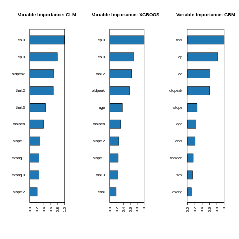
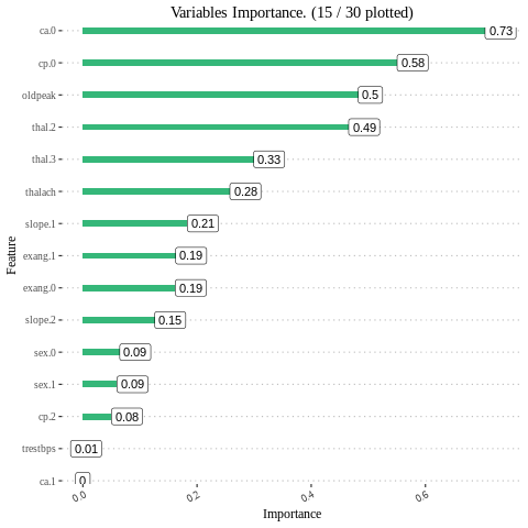
Feature interpretation {#glm-h2o-classification-binary-viz} Feature importance To identify the most influential variables we can use h2o’s variable importance plot. Variable importance is simply represented by the standardized coefficients. We see that response and Factor_D have the largest influence in increasing the probability of Approval whereas Factor_E.B and Factor_E.C. No have the largest influence in decreasing the probability of attrition.
%%R
par(mfrow=c(1,3))

h2o::h2o.varimp_plot(model_h2o_glm)
box()
#p2<-h2o.varimp_plot(aml@leader, num_of_features = 12)
h2o.varimp_plot(model_h2o_automl@leader)
box()


h2o.varimp_plot(model_h2o_gbm)
box()
#Varplot(feature=h2o_autodata$names,Importance=h2o_autodata$coefficients)
#gridExtra::grid.arrange(p1, nrow = 1)
%%R

h2o_glmdata<-data.frame(h2o.varimp(model_h2o_glm))

#h2o_glmdata

Varplot(feature=h2o_glmdata$variable,Importance=h2o_glmdata$relative_importance)
%%R


paste('accuracy :',mean(test$target==predictions$predict))


#class(predictions$predict%>%as_tibble())
[1] "accuracy : 0.906666666666667"
%%R

#as.data.frame(predictions)[[3L]]
head(predictions)
  predict        p0        p1
1       1 0.2321861 0.7678139
2       1 0.2905829 0.7094171
3       1 0.1771259 0.8228741
4       1 0.0918774 0.9081226
5       1 0.1243579 0.8756421
6       1 0.2017334 0.7982666
IML PROCEDURES
Steps to using iml:
-
Create a data frame with just the features (must be of class data.frame, cannot be an H2OFrame or other class).*
-
Create a vector with the actual responses (must be numeric - 0/1 for binary classification problems).*
-
iml has internal support for some machine learning packages (i.e. mlr, caret, randomForest). However, to use iml with several of the more popular packages being used today (i.e. h2o, ranger, xgboost) we need to create a custom function that will take a data set (again must be of class data.frame) and provide the predicted values as a vector.*
Create a predictor function for iml
%%R
h2o.no_progress()
# 1. create a data frame with just the features
features <- test_tbl %>% select(-target)

# 2. Create a vector with the actual responses
response <- as.numeric(test_tbl$target)

# 3. Create custom predict function that returns the predicted values as a
#    vector (probability of purchasing in our example)
pred  <- function(model, newdata)  {
  results <- as.data.frame(h2o.predict(model, as.h2o(newdata)))
  return(results[[3L]])
}

# example of prediction output
pred (model_h2o_automl@leader, features) %>% head()
[1] 0.7678139 0.7094171 0.8228741 0.9081226 0.8756421 0.7982666
Create an explainer function
%%R
predictor.AutoML <- Predictor$new(
  model = model_h2o_automl,
  data = features,
  y = response,
  predict.fun = pred,
  class = "classification"
  )
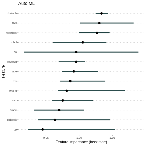
%%R

# compute feature importance with specified loss metric
#imp.AutoML <- FeatureImp$new(predictor.AutoML, loss = "mse")
imp = FeatureImp$new(predictor.AutoML, loss = "mae")
plot(imp)+ ggtitle("Auto ML")

# plot output
#plot(imp.AutoML) + ggtitle("Auto ML")


#gridExtra::grid.arrange(p1, p2, p3, nrow = 1)
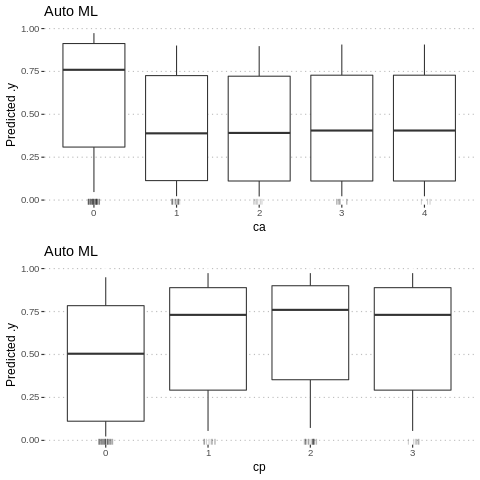
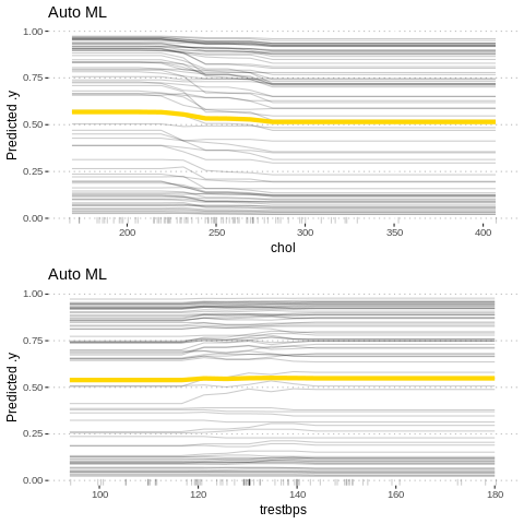
Partial Dependence Plot
Partial Dependence Plots (PDP) are one of the most popular methods for exploration of the relation between a continuous variable and the model outcome.
Function variable_response() with the parameter type = “pdp” calls pdp::partial() function to calculate PDP response.
%%R

p1<-Partial$new(predictor.AutoML, "ca") %>% plot() + ggtitle("Auto ML")


p2<-Partial$new(predictor.AutoML, "cp") %>% plot() + ggtitle("Auto ML")


gridExtra::grid.arrange(p1, p2, nrow = 2)
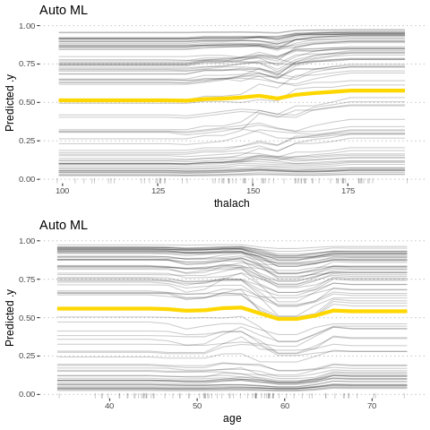
%%R


p3<-Partial$new(predictor.AutoML, "thalach") %>% plot() + ggtitle("Auto ML")


p4<-Partial$new(predictor.AutoML, "age") %>% plot() + ggtitle("Auto ML")


gridExtra::grid.arrange(p3,p4, nrow = 2)
%%R


p5<-Partial$new(predictor.AutoML, "chol") %>% plot() + ggtitle("Auto ML")

p6<-Partial$new(predictor.AutoML, "trestbps") %>% plot() + ggtitle("Auto ML")

gridExtra::grid.arrange(p5,p6, nrow = 2)
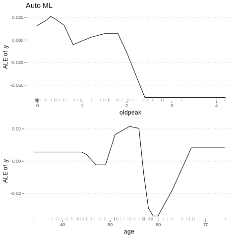
Feature effects
Besides knowing which features were important, we are interested in how the features influence the predicted outcome. The FeatureEffect class implements accumulated local effect plots, partial dependence plots and individual conditional expectation curves. The following plot shows the accumulated local effects (ALE) for the feature ‘lstat’. ALE shows how the prediction changes locally, when the feature is varied. The marks on the x-axis indicates the distribution of the ‘lstat’ feature, showing how relevant a region is for interpretation (little or no points mean that we should not over-interpret this region).
%%R

c1= FeatureEffect$new(predictor.AutoML, feature =c("age"))


c2 = FeatureEffect$new(predictor.AutoML, feature = "oldpeak")


gridExtra::grid.arrange(c2$plot()+ ggtitle("Auto ML"), c1$plot(),nrow = 2)
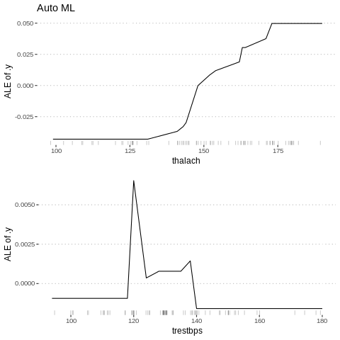
%%R


c3<-FeatureEffect$new(predictor.AutoML, "thalach")


c4<-FeatureEffect$new(predictor.AutoML, "trestbps")


gridExtra::grid.arrange(c3$plot()+ ggtitle("Auto ML"),
                        c4$plot(),nrow = 2)
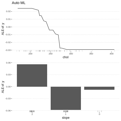
%%R


c5<-FeatureEffect$new(predictor.AutoML, "chol")


c6<-FeatureEffect$new(predictor.AutoML, "slope")


gridExtra::grid.arrange(c5$plot()+ ggtitle("Auto ML"), c6$plot(),nrow = 2)
#%%capture
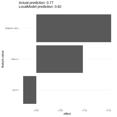
%%R
lime.explain = LocalModel$new(predictor.AutoML, x.interest = features[1,])
lime.explain$results
plot(lime.explain)
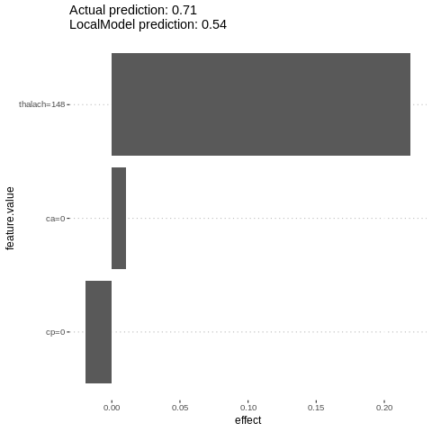
%%R

lime.explain$explain(features[2,])
plot(lime.explain)
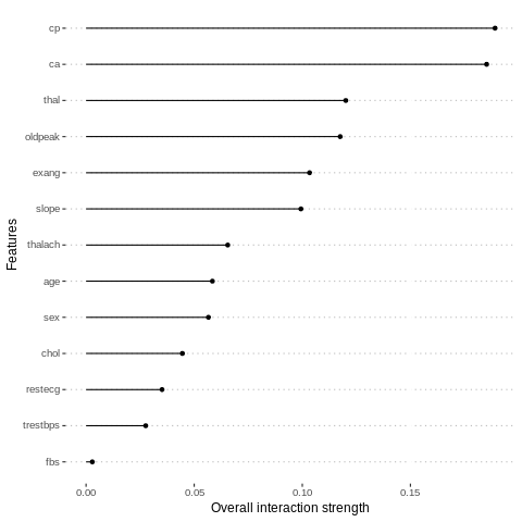
Measure interactions
We can also measure how strongly features interact with each other. The interaction measure regards how much of the variance of f(x) is explained by the interaction. The measure is between 0 (no interaction) and 1 (= 100% of variance of f(x) due to interactions). For each feature, we measure how much they interact with any other feature:
%%R
interact = Interaction$new(predictor.AutoML)
plot(interact)
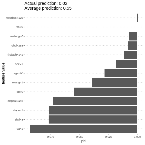
SHapley Additive exPlanations (SHAP) : Explain single predictions with game theory
An alternative for explaining individual predictions is a method from coalitional game theory named Shapley value. Assume that for one data point, the feature values play a game together, in which they get the prediction as a payout. The Shapley value tells us how to fairly distribute the payout among the feature values.
%%R

i=sample.int(dim(features)[1], 1)
shapley = Shapley$new(predictor.AutoML, x.interest = features[i,])
shapley$plot()
h2o
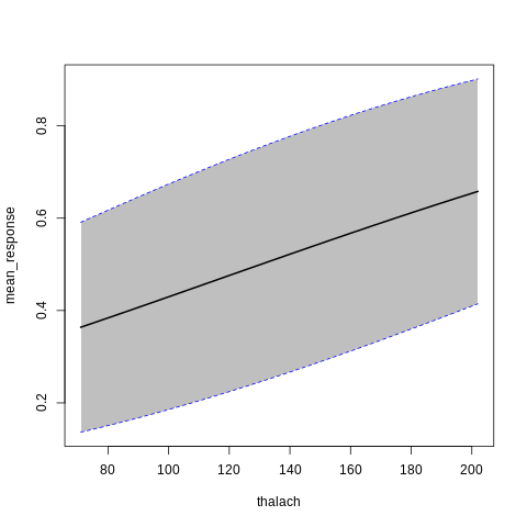
h2o Partial Dependence Plots
%%R
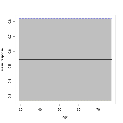
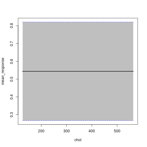
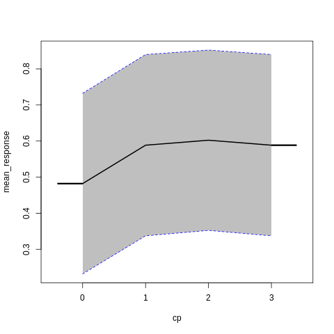
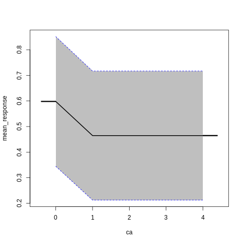
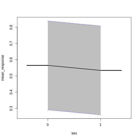
p7<-h2o.partialPlot(model_h2o_glm, data = train, cols = c("age","chol","cp","ca","sex","thalach"))
p7[[5]]
PartialDependence: Partial Dependence Plot of model GLM_model_R_1561909640968_8411 on column 'sex'
  sex mean_response stddev_response std_error_mean_response
1   0      0.564513        0.273718                0.018127
2   1      0.533609        0.273702                0.018126
DALEX
The explain() function
Steps to using DALEX:
-
The first step of using the DALEX package is to wrap-up the black-box model with meta-data that unifies model interfacing.
-
The next is to create an explainer function.
%%R
class(train_tbl$target)

train_tbl$target<-as.numeric(train_tbl$target)
%%R


custom_predict <- function(model, newdata)  {
                              newdata_h2o <- as.h2o(newdata)
                              res <- as.data.frame(h2o.predict(model, newdata_h2o))
                              return(as.numeric(res$predict))
     }


explainer_h2o_glm <- DALEX::explain(model = model_h2o_glm,
                             data = train_tbl[,-14],
                             y = train_tbl$target,
                             predict_function = custom_predict,
                             label = "h2o glm")


explainer_h2o_automl <- DALEX::explain(model = model_h2o_automl@leader,
                             data = train_tbl[,-14],
                             y = train_tbl$target,
                             predict_function = custom_predict,
                             label = "h2o automl")


explainer_h2o_gbm <- explain(model = model_h2o_gbm,
                            data = train_tbl[,-14],
                             y = train_tbl$target,
                             predict_function = custom_predict,
                             label = "h2o gbm")
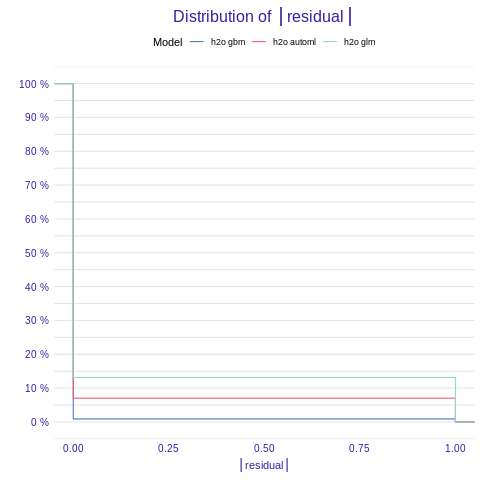
#### Model performance Function model_performance() calculates predictions and residuals for validation dataset.
%%R
mp_h2o_glm <- model_performance(explainer_h2o_glm)
mp_h2o_gbm <- model_performance(explainer_h2o_gbm)
mp_h2o_automl <- model_performance(explainer_h2o_automl)

plot(mp_h2o_glm, mp_h2o_gbm, mp_h2o_automl)
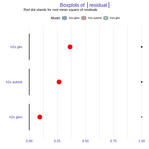
%%R
plot(mp_h2o_glm, mp_h2o_gbm, mp_h2o_automl, geom = "boxplot")
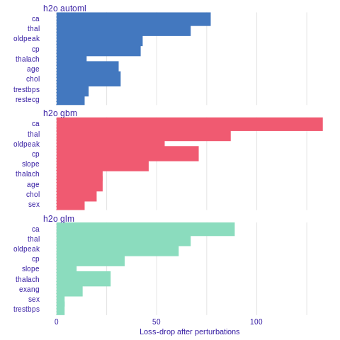
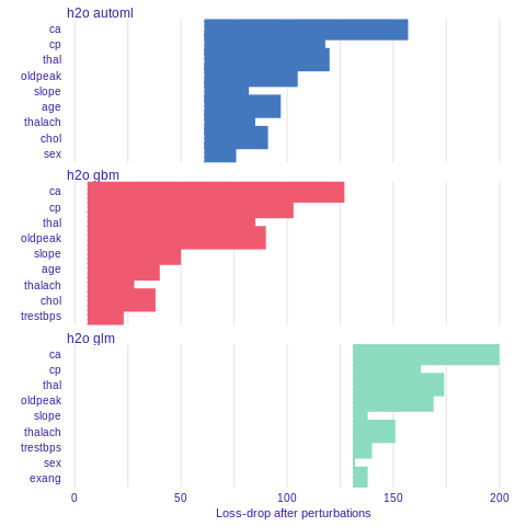
Variable importance
Using he DALEX package we are able to better understand which variables are important.
Model agnostic variable importance is calculated by means of permutations. We simply substract the loss function calculated for validation dataset with permuted values for a single variable from the loss function calculated for validation dataset.
This method is implemented in the variable_importance() function.
%%R
vi_h2o_glm <- variable_importance(explainer_h2o_glm, type="difference")
vi_h2o_gbm <- variable_importance(explainer_h2o_gbm, type="difference")
vi_h2o_automl <- variable_importance(explainer_h2o_automl, type="difference")
plot(vi_h2o_glm, vi_h2o_gbm, vi_h2o_automl)
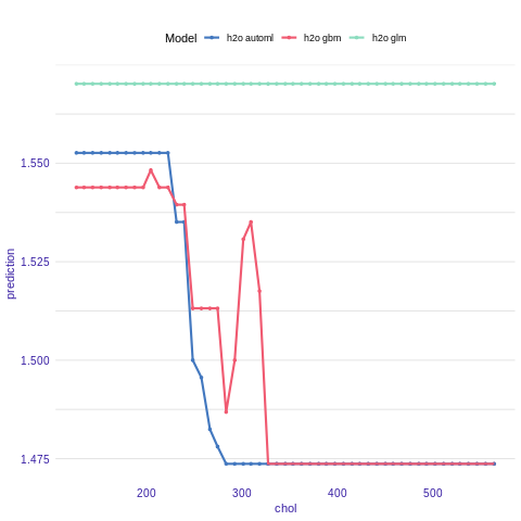
Partial Dependence Plot
Partial Dependence Plots (PDP) are one of the most popular methods for exploration of the relation between a continuous variable and the model outcome.
Function variable_response() with the parameter type = “pdp” calls pdp::partial() function to calculate PDP response.
%%R
#install.packages("factorMerger")
#devtools::install_github("MI2DataLab/factorMerger", build_vignettes = FALSE)
#install.packages("units")
#library(units)
#library(factorMerger)
pdp_h2o_glm <- variable_response(explainer_h2o_glm, variable = "chol")
pdp_h2o_gbm <- variable_response(explainer_h2o_gbm, variable = "chol")
pdp_h2o_automl <- variable_response(explainer_h2o_automl, variable = "chol")

plot(pdp_h2o_glm, pdp_h2o_gbm, pdp_h2o_automl)
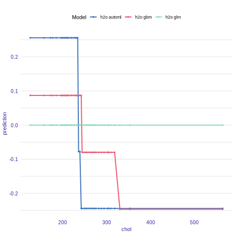
Acumulated Local Effects plot
Acumulated Local Effects (ALE) plot is the extension of PDP, that is more suited for highly correlated variables.
Function variable_response() with the parameter type = “ale” calls ALEPlot::ALEPlot() function to calculate the ALE curve for the variable construction.year.
%%R

ale_h2o_glm <- variable_response(explainer_h2o_glm, variable = "chol", type = "ale")
ale_h2o_gbm <- variable_response(explainer_h2o_gbm, variable = "chol", type = "ale")
ale_h2o_automl <- variable_response(explainer_h2o_automl, variable = "chol", type = "ale")

plot(ale_h2o_glm,ale_h2o_automl,ale_h2o_gbm)
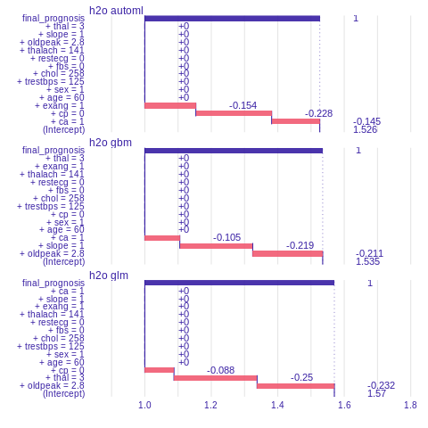
Prediction understanding
The function prediction_breakdown() is a wrapper around a breakDown package. Model prediction is visualized with Break Down Plots, which show the contribution of every variable present in the model. Function prediction_breakdown() generates variable attributions for selected prediction. The generic plot() function shows these attributions.
%%R
library("breakDown")


i=sample.int(dim(features)[1], 1)
pb_h2o_glm <- prediction_breakdown(explainer_h2o_glm, observation = as.data.frame(test[i,]))
pb_h2o_gbm <- prediction_breakdown(explainer_h2o_gbm, observation =as.data.frame(test[i,]))
pb_h2o_automl <- prediction_breakdown(explainer_h2o_automl, observation = as.data.frame(test[i,]))

plot(pb_h2o_glm, pb_h2o_gbm, pb_h2o_automl)
Variable importance
Using he DALEX package we are able to better understand which variables are important.
Model agnostic variable importance is calculated by means of permutations. We simply substract the loss function calculated for validation dataset with permuted values for a single variable from the loss function calculated for validation dataset.
This method is implemented in the variable_importance() function.
%%R

vi_h2o_glm <- variable_importance(explainer_h2o_glm)

vi_h2o_gbm <- variable_importance(explainer_h2o_gbm)

vi_h2o_automl <- variable_importance(explainer_h2o_automl)

#We can compare all models using the generic plot() function.

plot(vi_h2o_glm, vi_h2o_gbm, vi_h2o_automl)
%%R

summary(explainer_h2o_glm)
                 Length Class            Mode
model              1    H2OBinomialModel S4
data              13    data.frame       list
y                228    -none-           numeric
predict_function   1    -none-           function
link               1    -none-           function
class              1    -none-           character
label              1    -none-           character
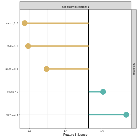
Explaining classification models with localModel package
Local prediction analysis can be performed by using the localModel package in R. The package works similarly to the lime package.
%%R
install.packages('localModel')
library(DALEX)
library(localModel)


i=sample.int(dim(features)[1], 1)
new_observation <-as.data.frame(test[i,])

model_lok <- individual_surrogate_model(explainer_h2o_automl, new_observation,
                                        size = 500, seed = 17)
plot(model_lok)
%%R
h2o.shutdown(prompt = TRUE)