Statistical Methods For Data Drift Detection
Introduction
Data quality issues account for majority of machine learning model flaws. Monitoring and detecting changes in data is commonly used to identify causes of model performance degradation, model drift, decay or staleness. One of the most important components of machine learning operations is model performance monitoring after model deployment. Monitoring and detecting concept drift is commonly used to identify causes of model performance degradation. Concept drift entails changes in underlying distribution of data over time.
Why Model Monitoring?
Monitoring procedures will help to continuously track the health of the machine learning model against a set of key indicators and generate event-based alerts. When a machine learning model is deployed in production, it can start degrading in quality fast and without warning until it is too late. That is why model monitoring is a crucial step in the ML model life cycle and a critical piece of Model Ops. Data Skew refers to differences between two static data versions/sources such as training set and serving set.
Concept drift Concept drift means the statistical relationship between the target variable and the features used in the model for prediction has changed over time. If concept drift occurs, the nature of the statistical relationship between the target and features may no longer exist which causes the decision boundary to also change and cause the model to produce poor predictions. Machine learning under concept drift involves three components: drift detection( whether drift occurs),drift understanding(when,how, where it occurs) and drift adaption(reaction to the existence of drift)
Causes od Data Drift
-
Change in relation between features, or covariate shift.
-
Unexpected changes in the macro economic environment such COVID-19’s impact on the economy.
-
Natural drift in data such as seasonal changes with temperature.
-
Data quality issues such as a broken-down server that does not transmit or store data.
Examples of Data Drift
- A change in ground truth or input data distribution e.g. change in customer preferences such as in fashion styles, from a natural distater pandemic, product launch in a new market etc.
General Framework For Drift Detection
The framework for drift detection consist of four stages namely data
- retrieval
- data modeling
- test statistics calculation and
- hypothesis testing.
Data retrieval involves getting the data from the storage location ontoa processing platform. Data modeling involves selecting those features that will significantly impact the system when they drift. The dissimilarity measurements involve designing a metric such as distance or test-statistic to quantify the level of drift and a test-statistics for the hypothesis test.Choosing an appropriate and robust measure of dissimilarity is an open question. The concept drift detect significance test can be seen as a two sample test of difference in distribution between two samples.
Types of Concept Drfit
Concept drift can be distinguished as four types namely sudden, gradual,incremental and reccurring. Research on the first three explores how to minimize drop in model performance and achieve the fastest recovery rate during the concept transformation process. The fourth kind emphasizes how to find the best matched historical concepts with the shortest time
Concept Drift Detection Algorithms
Error rate-based drift detection
This consist of a class of algorithms that track changes in error rate by classifiers online. A significant change in error rate corresponds to the occurrence of drift. Example Implementation of this algorithm can be found in the following:
- Local Drift Detection (LLDD)
- Early Drift Detection Method (EDDM)
- Heoffding’s inequality based Drift Detection Method (HDDM)
- Fuzzy Windowing Drift Detection Method (FW-DDM)
-
Dynamic Extreme Learning Machine (DELM)
- ADaptive Windowing (ADWIN) is popular two time windowing drift detection algorithm. Unlike several counterparts, it does not require the window size to be specified beforehand but computes a optimal window size by examining all possible window cuts once the total size n of a sufficiently large window W is specified. The test statistic is the difference of the two sample means
| $\theta_{ADWIN} = | \hat{\mu_{hist}}-\hat{\mu_{new}} | $ |
Data Distribution-based Drift Detection
Data distribution based drift algorithms algorithms use distance metrics to quantify the dissimilarity between historical and new data over time. A statistically significant distance between the two data distributions indicates the time is right for model upgrade. This addresses concept drift from its root source which is a shift in distribution of data. These algorithms require time windows for historical and new data to be pre-specified.
Similar distribution-based drift detection methods or algorithms are:
- Statistical Change Detection for multidimensional data (SCD).
- Competence Model-based drift detection (CM)
- a prototype-based classification model for evolving data streams called SyncStream.
- PCA-based change detection framework (PCA-CD)
- Equal Density Estimation (EDE)
- Least Squares Density
- Difference-based Change Detection Test (LSDD-CDT)
- Incremental version of LSDD-CDT (LSDD-INC) and Local Drift Degree-based Density Synchronized Drift Adaptation (LDD-DSDA).
Multiple Hypothesis Test Drift Detection
They combine ideas from both error-rate and data distribution drift and use multiple hypothesis test to detect concept drift. This method employs Principal Component Analysis from feature extraction,drift is then detected in each component and also among combinations of the feature space. Implementations include:
- Linear Four Rate drift detection (LFR)
- three-layer drift detection, based on Information Value and Jaccard similarity (IV-Jac)
- Ensemble of Detectors (e-Detector)
- Hierarchical Linear Four Rate (HLFR)
- Hierarchical Hypothesis Testing with Classification Uncertainty (HHT-CU).
the features extracted by Principal Component Analysis (PCA)
Strategies for Detecting Drift
Population Stability Index(PSI)
The Population Stability Index (PSI) is a measure of the degree to which the distribution of some variable in a population changes between two time periods, say T1 and T2. It is calculated by comparing a score variable divided into several buckets where the number of buckets is discretionary. The contribution of each bucket is computed as the arithmetic change (P2 - P1) in the percentage of the population assigned to the bucket, weighted by the log of the geometric change, i.e. the ratio (P2 / P1) of the final percentage to the initial percentage. Rule of thumb for making decisions about PSI available in statistical literature is listed below:
- If PSI < 0.1, there is no significant change in the data and no action is required.
- If 0.1 < PSI < 0.25, there is minor change in the data and some further monitoring is necessary.
- If PSI > 0.25, there is a major change in the data distribution and appropriate investigation should be initiated.
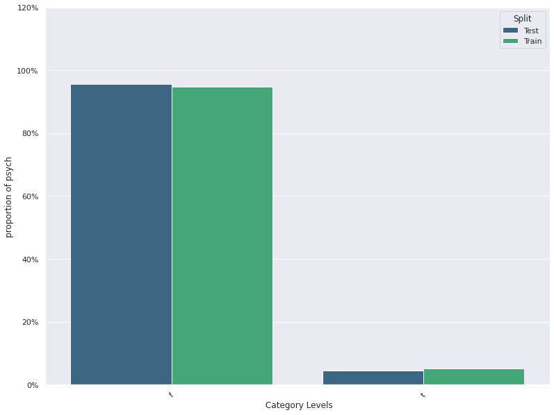
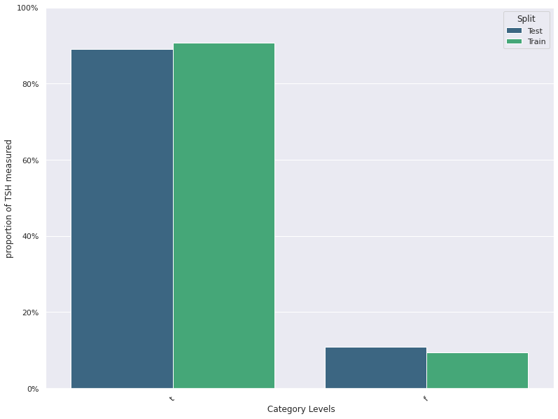
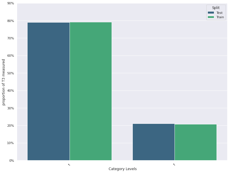
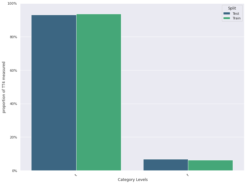
Feature Distribution Plots :
For categorical and continuous features:
- A feature distribution plot can be used to compare the empirical feature distribution of a feature at two or multiple time points (Train distribution vs server/Prediction data distribution).
- The kernel density estimate is used for continuous features and histograms are used for categorical features.
import pandas as pd
import numpy as np
from sklearn.model_selection import train_test_split
import numpy as np # linear algebra
import pandas as pd # data processing, CSV file I/O (e.g. pd.read_csv)
from pandas.tseries.holiday import USFederalHolidayCalendar as calendar
import os
import matplotlib.pyplot as plt
import seaborn as sns
import re
import gensim
import plotly
from plotly import graph_objs as go
import plotly.express as px
import plotly.figure_factory as ff
from collections import Counter
from sklearn.model_selection import train_test_split
from sklearn.feature_extraction.text import CountVectorizer
from sklearn.linear_model import LogisticRegression
from sklearn.metrics import roc_auc_score
from sklearn.metrics import confusion_matrix
from tqdm import tqdm
import itertools
import collections
from xgboost import XGBClassifier
import xgboost as xgb
import warnings
from tqdm.notebook import tqdm
tqdm.pandas(desc="Completed") # add progressbar to pandas, use progress_apply instead apply
from ipywidgets import interact #interactive plots
#from IPython.display import clear_output
from datetime import datetime
#import pandas_profiling
#import sweetviz as sv
from sklearn.impute import SimpleImputer
from sklearn.ensemble import RandomForestRegressor
import missingno as msno
# activate R magic
import rpy2
import seaborn as sns
import matplotlib.pyplot as plt
import sklearn
import random

from sklearn.preprocessing import OrdinalEncoder
from sklearn.preprocessing import LabelEncoder
from sklearn.model_selection import train_test_split

#!pip install Boruta
#from boruta import BorutaPy
from sklearn.ensemble import RandomForestClassifier
from sklearn.ensemble import ExtraTreesClassifier
from sklearn.feature_selection import RFE

from sklearn.pipeline import Pipeline

from sklearn import metrics
from sklearn.model_selection import cross_val_score
from sklearn.model_selection import GridSearchCV, RandomizedSearchCV

# !pip install imblearn
#from imblearn.over_sampling import SMOTE
from collections import Counter

#from imblearn.under_sampling import RandomUnderSampler
#from imblearn.over_sampling import RandomOverSampler
#from imblearn.pipeline import make_pipeline
#!pip install lightgbm
import lightgbm as lgb
import pickle
#!pip install bayesian-optimization
#from bayes_opt import BayesianOptimization

#!pip install hyperopt
from hyperopt import fmin, tpe, hp,Trials
import matplotlib.ticker as mtick
#!pip install scikit-plot
#import scikitplot as skplt
import gc
import glob
warnings.filterwarnings("ignore")
#%load_ext rpy2.ipython
%matplotlib inline
%autosave 5

pd.set_option('display.max_columns', None)
pd.set_option('display.max_rows', None)

column_names = ['age',	'workclass',	'fnlwgt',	'education',
'education-num',	'marital-status',	'occupation',
	'relationship',	'race',	'sex',	'capital-gain',
  	'capital-loss',	'hours-per-week',	'native-country',	'label']

column_names =['age','sex','on thyroxine','query on thyroxine','on antithyroid medication','sick',
'pregnant','thyroid surgery','I131 treatment','query hypothyroid','query hyperthyroid','lithium',
'goitre','tumor','hypopituitary','psych','TSH measured','TSH','T3 measured','T3','TT4 measured',
'TT4','T4U measured','T4U','FTI measured','FTI','TBG measured','TBG','referral source','Target']
# Read in the training and evaluation datasets
#df_train = pd.read_csv('/content/drive/MyDrive/Data/adult.data.zip', skipinitialspace=True,header=None,names=column_names)
#df = pd.read_csv('/content/drive/MyDrive/Data/adult.test', skipinitialspace=True,header=None,names=column_names)
df = pd.read_csv('/Data/allbp.data', skipinitialspace=True,header=None,names=column_names)
# Split the dataset. Do not shuffle for this demo notebook.
train_df, test_df = train_test_split(df, test_size=0.5, shuffle=False)
#train_df, val_df = train_test_split(train_df, test_size=0.2, shuffle=False)
#print(f"size of training set : {train_df.shape}")
#print(f"size of validation set : {val_df.shape}")
#print(f"size of test set : {test_df.shape}")
print(f"size of train set : {train_df.shape}")
print(f"size of  test set : {test_df.shape}")
print(f"size of full set : {df.shape}")
print(len(column_names))
test_df.head()
Autosaving every 5 seconds
size of train set : (1400, 30)
size of  test set : (1400, 30)
size of full set : (2800, 30)
30
| age | sex | on thyroxine | query on thyroxine | on antithyroid medication | sick | pregnant | thyroid surgery | I131 treatment | query hypothyroid | query hyperthyroid | lithium | goitre | tumor | hypopituitary | psych | TSH measured | TSH | T3 measured | T3 | TT4 measured | TT4 | T4U measured | T4U | FTI measured | FTI | TBG measured | TBG | referral source | Target | |
|---|---|---|---|---|---|---|---|---|---|---|---|---|---|---|---|---|---|---|---|---|---|---|---|---|---|---|---|---|---|---|
| 1400 | 62 | M | f | f | f | f | f | f | f | f | f | f | f | f | f | f | t | 1.4 | t | 3.9 | t | 97 | t | 0.84 | t | 115 | f | ? | other | negative.|68 |
| 1401 | 57 | F | t | f | f | f | f | f | f | f | f | f | f | f | f | f | t | 0.1 | t | 2.2 | t | 150 | t | 1.01 | t | 149 | f | ? | SVI | negative.|183 |
| 1402 | 65 | F | t | f | f | f | f | f | f | f | f | f | f | f | f | f | t | 2.5 | f | ? | t | 137 | t | 1.06 | t | 129 | f | ? | other | negative.|2930 |
| 1403 | 90 | M | f | f | f | f | f | f | f | f | f | f | f | f | f | f | t | 0.15 | t | 1.7 | t | 118 | t | 0.82 | t | 144 | f | ? | SVI | negative.|1830 |
| 1404 | 68 | M | f | f | f | f | f | f | f | f | f | f | f | f | f | f | t | 1.4 | t | 1.9 | t | 98 | t | 0.82 | t | 118 | f | ? | other | negative.|1467 |
#df.iloc[:,29].nunique()
df.apply(lambda x : x.nunique())
age                            94
sex                             3
on thyroxine                    2
query on thyroxine              2
on antithyroid medication       2
sick                            2
pregnant                        2
thyroid surgery                 2
I131 treatment                  2
query hypothyroid               2
query hyperthyroid              2
lithium                         2
goitre                          2
tumor                           2
hypopituitary                   2
psych                           2
TSH measured                    2
TSH                           264
T3 measured                     2
T3                             65
TT4 measured                    2
TT4                           218
T4U measured                    2
T4U                           139
FTI measured                    2
FTI                           210
TBG measured                    1
TBG                             1
referral source                 5
Target                       2800
dtype: int64
train_df.drop(['TBG measured','TBG'],inplace=True,axis=1)
test_df.drop(['TBG measured','TBG'],inplace=True,axis=1)
#print(df_train.dtypes)

#numeric_cols = df_train.select_dtypes(include=np.number).columns


#categorical_cols

numeric_cols  = ['age','TSH','T3','TT4','T4U','FTI']


for col in numeric_cols:
    train_df[col]  = pd.to_numeric(train_df[col],errors= 'coerce')
    test_df[col]  = pd.to_numeric(test_df[col],errors= 'coerce')


categorical_cols = train_df.select_dtypes(exclude=np.number).columns

categorical_cols = ['sex', 'on thyroxine', 'query on thyroxine',
       'on antithyroid medication', 'sick', 'pregnant', 'thyroid surgery',
       'I131 treatment', 'query hypothyroid', 'query hyperthyroid', 'lithium',
       'goitre', 'tumor', 'hypopituitary', 'psych', 'TSH measured',
       'T3 measured', 'TT4 measured', 'T4U measured', 'FTI measured',
        'referral source']


train_df[categorical_cols].head()
| sex | on thyroxine | query on thyroxine | on antithyroid medication | sick | pregnant | thyroid surgery | I131 treatment | query hypothyroid | query hyperthyroid | lithium | goitre | tumor | hypopituitary | psych | TSH measured | T3 measured | TT4 measured | T4U measured | FTI measured | referral source | |
|---|---|---|---|---|---|---|---|---|---|---|---|---|---|---|---|---|---|---|---|---|---|
| 0 | F | f | f | f | f | f | f | f | f | f | f | f | f | f | f | t | t | t | t | t | SVHC |
| 1 | F | f | f | f | f | f | f | f | f | f | f | f | f | f | f | t | t | t | f | f | other |
| 2 | M | f | f | f | f | f | f | f | f | f | f | f | f | f | f | t | f | t | t | t | other |
| 3 | F | t | f | f | f | f | f | f | f | f | f | f | f | f | f | t | t | t | f | f | other |
| 4 | F | f | f | f | f | f | f | f | f | f | f | f | f | f | f | t | t | t | t | t | SVI |
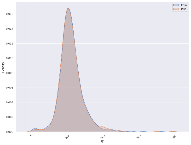
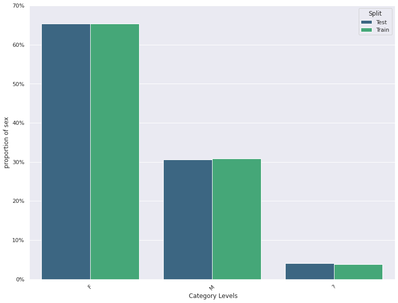
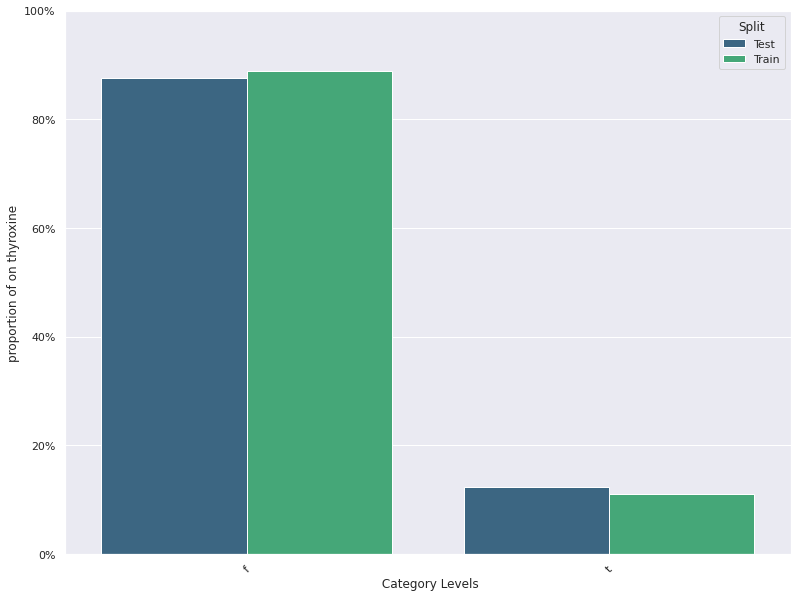
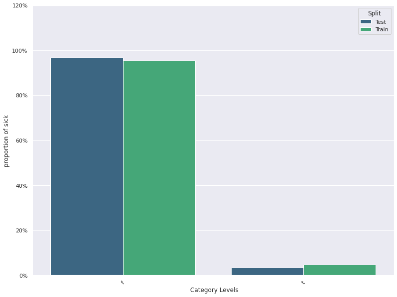
'''
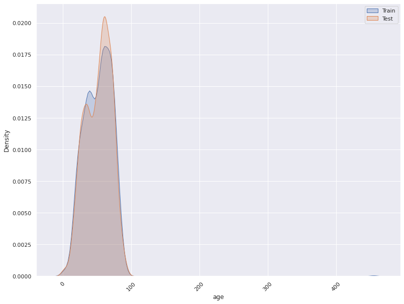
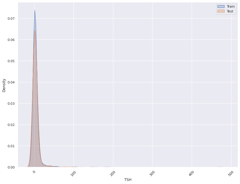
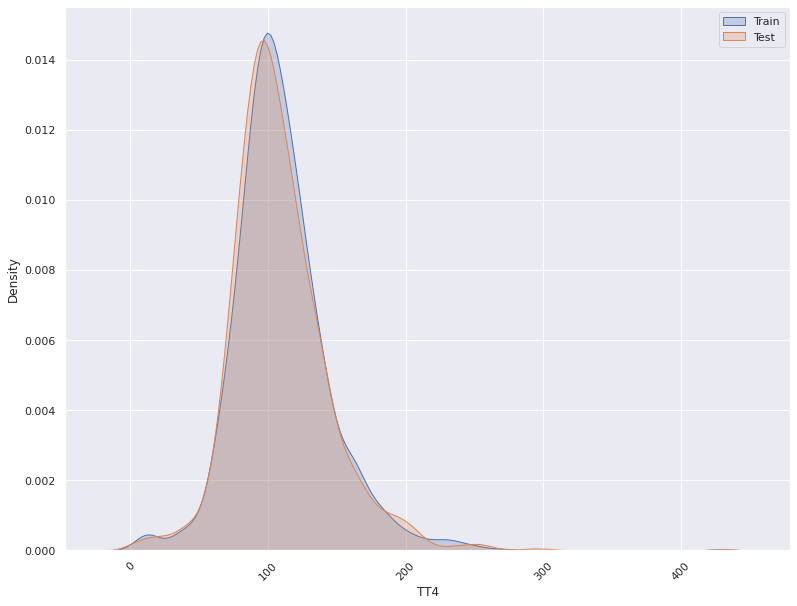
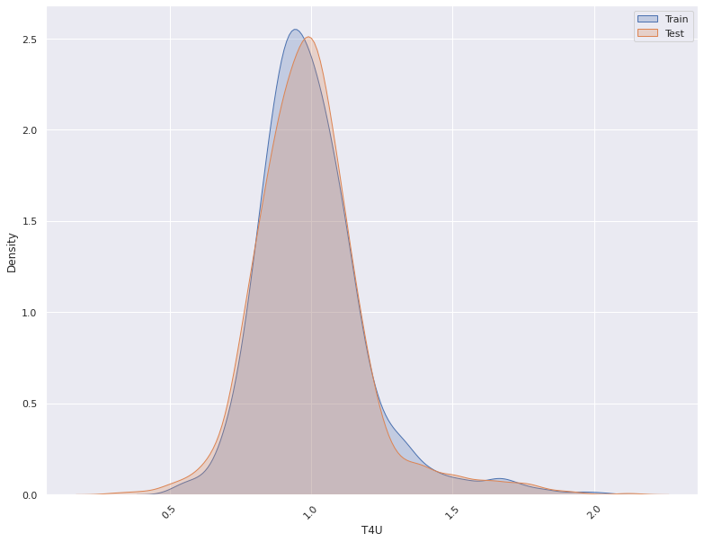
1. This plots the distribution of a feature in a training data and test data.
The plot allows us to visually inspect if there is difference in the distribution
of the feature in the two datasets
2. Example of usage below:
Kernel Density Plot
https://seaborn.pydata.org/generated/seaborn.kdeplot.html
Example
DistributionPlot(data=data,categorical_cols= categorical_cols,continuous_columns= numeric_cols,
save_location=save_location,split_column='Split').feature_dist_plot()
`
- For continuous features, the kernel density plot of the feature is plotted whereas for categorical features the
histogram is plotted.
- split_column splits the input dataset into two parts, the training/reference and the test/deployment dataset
'''
import seaborn as sns
sns.set(rc = {'figure.figsize':(13,10)})
import matplotlib.ticker as mtick
save_location = '/drift/'
def count_plot(column):
d1 = pd.DataFrame(test_df[column].value_counts()/test_df[column].shape[0]).reset_index().rename(columns={'index':'Value'})
d1["Split"] = "Train"
d2 = pd.DataFrame(val_df[column].value_counts()/val_df[column].shape[0]).reset_index().rename(columns={'index':'Value'})
d2["Split"] = "Validation"
d3 = pd.DataFrame(test_df[column].value_counts()/test_df[column].shape[0]).reset_index().rename(columns={'index':'Value'})
d3["Split"] = "Test"
d = pd.concat([d1,d2,d3])
ax = sns.barplot(x="Value", y = column, data=d,hue="Split", palette="viridis")
plt.savefig(save_location+f'{column}.png')
plt.ylabel(f'proportion of {column}')
plt.xlabel(" Category Levels")
plt.xticks(rotation=45)
plt.yticks(plt.yticks()[0], ['{:,.0%}'.format(x) for x in plt.yticks()[0]])
class DistributionPlot:
# constructor of Main class
def __init__(self, data, categorical_cols, continuous_columns, save_location, split_column):
# Initialization of the Strings
self.data = data
self.categorical_cols = categorical_cols
self.continuous_columns = continuous_columns
self.save_location = save_location
self.split_column = split_column
def feature_dist_plot(self):
Train_Data = self.data.loc[data[self.split_column] == 'Train']
Val_Data = self.data.loc[data[self.split_column] == 'Validation']
Test_Data = self.data.loc[data[self.split_column] == 'Test']
for i in self.continuous_columns:
plt.figure()
fig = sns.kdeplot(x=Train_Data[i], label='Train', shade=True)
fig = sns.kdeplot(x= Val_Data[i], label='Validation', shade=True)
fig = sns.kdeplot(x=Test_Data[i], label='Test', shade=True)
fig.legend()
plt.xticks(rotation=45)
plt.savefig(self.save_location+f'{i}.png')
plt.show()
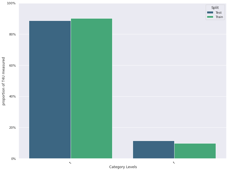
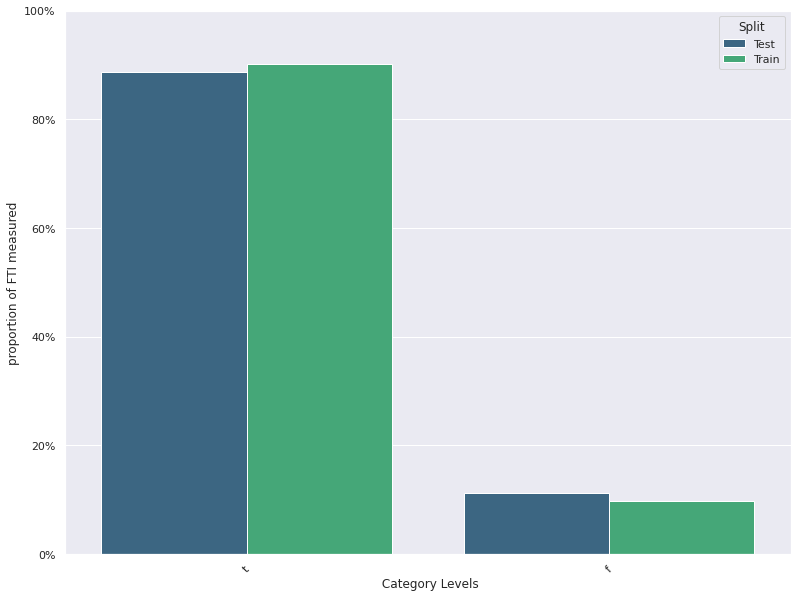
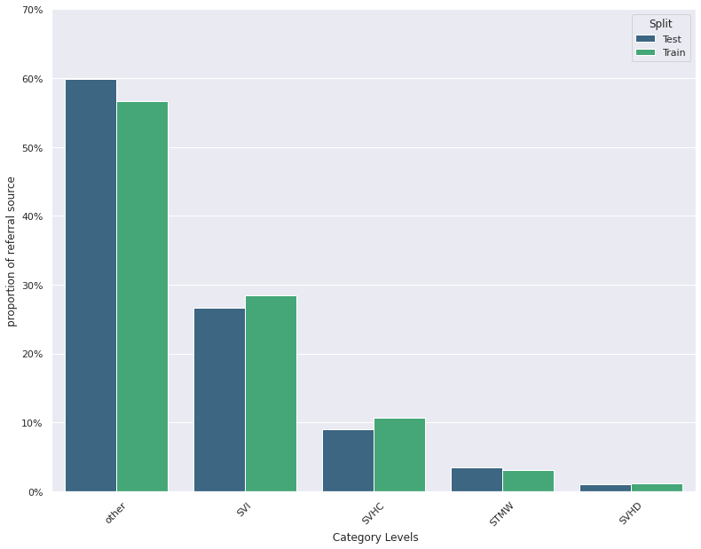
for i in self.categorical_cols:
plt.figure()
d1 = pd.DataFrame(Test_Data[i].value_counts()/Test_Data[i].shape[0]).reset_index().rename(columns={'index':'Value'})
d1["Split"] = "Test"
d2 = pd.DataFrame(Val_Data[i].value_counts()/Val_Data[i].shape[0]).reset_index().rename(columns={'index':'Value'})
d2["Split"] = "Validation"
d3 = pd.DataFrame(Train_Data[i].value_counts()/Train_Data[i].shape[0]).reset_index().rename(columns={'index':'Value'})
d3["Split"] = "Train"
d = pd.concat([d1,d2,d3])
ax = sns.barplot(x="Value", y = i, data=d,hue="Split", palette="viridis")
plt.savefig(save_location+f'{i}.png')
plt.ylabel(f'proportion of {i}')
plt.xlabel(" Category Levels")
plt.yticks(plt.yticks()[0], ['{:,.0%}'.format(x) for x in plt.yticks()[0]])
plt.xticks(rotation=45)
plt.show()
return fig
save_location = '/drift/'
train_df['Split']= "Train"
#val_df['Split'] = "Validation"
test_df['Split'] = "Test"
for name in numeric_cols:
train_df[name] = pd.to_numeric(train_df[name])
train_df[name] = train_df[name].astype(float)
#val_df[name] = pd.to_numeric(val_df[name])
#val_df[name] = val_df[name].astype(float)
test_df[name] = pd.to_numeric(test_df[name])
test_df[name] = test_df[name].astype(float)
data = pd.concat([train_df,test_df])
data[numeric_cols].dtypes
#catcol = cat_col2 + boolean_numeric
DistributionPlot(data=data,categorical_cols= categorical_cols,continuous_columns= numeric_cols,
save_location=save_location,split_column='Split').feature_dist_plot()


Statistical Test For Concept Drift Detection
Paired T- test
- Test whether the mean difference between pairs of measurements is zero or not.
-
The Paired Samples T-Test compares the means for two related (paired) units on a continuous outcome that is normally distributed.
- $ H_{0} $ : $ \mu_{1}-\mu_{2} =0 $ The difference in mean of two populations is equal to 0.
- $ H_{1} $ : $ \mu_{1} - \mu_{2} \neq 0 $ The difference in mean of two populations is different from 0.
Kolmogorov-Smirnov Test :
- The K-S test is a nonparametric test that compares the cumulative distributions of two random variables.
- This can be used to test for significant difference between a feature in two time periods.
-
This test is for continuous features.
- $ H_{0} $: The feature distribution in the two populations are equal versus
- $ H_{1} $: The feature distribution in the two populations are not equal.
from scipy import stats
import numpy as np

def kolmogorovsmirnovtest(train_df,test_df,columns,significance_level = 0.05):
    Test_Statistic = []
    P_Value = []
    Feature = list()
    for col in columns:
        #val = stats.ks_2samp(np.array(train_df[col]), np.array(test_df[col]))
        val = stats.ks_2samp(train_df[col], test_df[col],mode="exact")
        Test_Statistic.append(val[0])
        P_Value.append(val[1])
        Feature.append(col)

    output= pd.DataFrame()
    output['Feature'] = Feature
    output['Test_Statistic'] =Test_Statistic
    output['P_Value'] = P_Value
    output['Decision']  = np.where(output['P_Value'] < significance_level,'Reject H0 : significant Difference','Do Not Reject H0 : No significant Difference')

    return output


numeric_cols = train_df.select_dtypes(include=np.number).columns


kolmogorovsmirnovtest(train_df= train_df,test_df= test_df,columns= numeric_cols,significance_level = 0.05)
| Feature | Test_Statistic | P_Value | Decision | |
|---|---|---|---|---|
| 0 | age | 0.032143 | 0.464819 | Do Not Reject H0 : No significant Difference |
| 1 | TSH | 0.032857 | 0.436584 | Do Not Reject H0 : No significant Difference |
| 2 | T3 | 0.035000 | 0.357931 | Do Not Reject H0 : No significant Difference |
| 3 | TT4 | 0.042143 | 0.166343 | Do Not Reject H0 : No significant Difference |
| 4 | T4U | 0.024286 | 0.803661 | Do Not Reject H0 : No significant Difference |
| 5 | FTI | 0.020714 | 0.924908 | Do Not Reject H0 : No significant Difference |
Anderson-Darling Test for k-samples
- It is a modification of the Kolmogorov-Smirnov (K-S) test.
- The populations from which two or more groups of data were drawn are identical.
- The distribution function of that population do not have to be specified.
-
Three versions of the k-sample Anderson-Darling test: one for continuous distributions and two for discrete distributions.
- $ H_{0} $ : k-samples are drawn from the same population.
- $ H_{1} $ : The populations from which two or more groups of data were drawn are not identical.
from scipy import stats
import numpy as np
#The critical values for significance levels 25%, 10%, 5%, 2.5%, 1%, 0.5%, 0.1%.
out = stats.anderson_ksamp([train_df['age'],test_df['age']])
#print(out[1][-2])
out
Anderson_ksampResult(statistic=-0.4825370980213063, critical_values=array([0.325, 1.226, 1.961, 2.718, 3.752, 4.592, 6.546]), significance_level=0.25)
Wilcoxon-Signed Rank Test
-
It tests whether the distribution of the differences of two paired samples is symmetric about zero or equivalently the null hypothesis that two related paired samples originate from the same distribution. It is a non-parametric version of the paired T-test (Difference in locationparameter) for continuous variables.
- $ H_{0} $ : The difference between the two populations follows a symmetric distribution around zero.
- $ H_{1} $ : The difference between the pairs does not follow a symmetric distribution around zero.
The null hypothesis can be rejected if the p-value is less than the significance level(0.05).
If the interest is in detecting a positive or negative shift in one population from the other, then the hypothesis can be specified as one-sided. The test procedure combines the observations from the two pools into one sample and then by keeping track of which sample each observation comes from, rank the lowest to highest from 1 to n1+n2, respectively.
from scipy import stats
import numpy as np
import  scipy

def wilcoxontest(train_df,test_df,columns,significance_level = 0.05):
    Test_Statistic = []
    P_Value = []
    Feature = list()
    for col in columns:
        #val = stats.ks_2samp(np.array(train_df[col]), np.array(test_df[col]))
        val = scipy.stats.wilcoxon(train_df[col], test_df[col],mode="auto")
        Test_Statistic.append(val[0])
        P_Value.append(val[1])
        Feature.append(col)

    output= pd.DataFrame()
    output['Feature'] = Feature
    output['Test_Statistic'] =Test_Statistic
    output['P_Value'] = P_Value
    output['Decision']  = np.where(output['P_Value'] < significance_level,'Reject H0 : significant Difference','Do Not Reject H0 : No significant Difference')

    return output


wilcoxontest(train_df= train_df,test_df= test_df,columns= numeric_cols,significance_level = 0.05)
| Feature | Test_Statistic | P_Value | Decision | |
|---|---|---|---|---|
| 0 | age | 465252.5 | 5.364083e-01 | Do Not Reject H0 : No significant Difference |
| 1 | TSH | 314479.0 | 2.334189e-29 | Reject H0 : significant Difference |
| 2 | T3 | 170417.5 | 4.000233e-90 | Reject H0 : significant Difference |
| 3 | TT4 | 352276.5 | 1.393954e-17 | Reject H0 : significant Difference |
| 4 | T4U | 294315.5 | 2.610237e-35 | Reject H0 : significant Difference |
| 5 | FTI | 299891.5 | 3.434791e-34 | Reject H0 : significant Difference |
scipy.stats.wilcoxon(train_df['age'], test_df['age'],mode="auto")
WilcoxonResult(statistic=465252.5, pvalue=0.5364083181880943)
Mann–Whitney U test
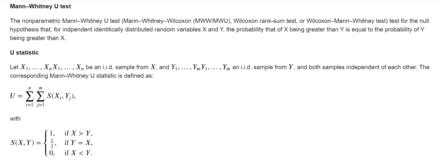
$ H_0 $: the distributions of both populations are identical
$ H_1 $: the distributions are not identical.
train_df.fillna(0)
from scipy.stats import mannwhitneyu
U1, p = mannwhitneyu(train_df['age'].fillna(0), test_df['age'].fillna(0), method="auto")
print(U1)
print(p)
mannwhitneyu(train_df['age'].fillna(0), test_df['age'].fillna(0), method="auto")
975127.5
0.8197947010766226


MannwhitneyuResult(statistic=975127.5, pvalue=0.8197947010766226)
from scipy import stats
import numpy as np
from scipy.stats import mannwhitneyu

def mannwhitneyu_test(train_df,test_df,columns,significance_level = 0.05):
    Test_Statistic = []
    P_Value = []
    Feature = list()
    for col in columns:
        #val = stats.ks_2samp(np.array(train_df[col]), np.array(test_df[col]))
        #val = stats.ks_2samp(train_df[col], test_df[col],mode="exact")
        val= mannwhitneyu(train_df[col].fillna(0), test_df[col].fillna(0), method="auto")
        Test_Statistic.append(val[0])
        P_Value.append(val[1])
        Feature.append(col)

    output= pd.DataFrame()
    output['Feature'] = Feature
    output['Test_Statistic'] =Test_Statistic
    output['P_Value'] = P_Value
    output['Decision']  = np.where(output['P_Value'] < significance_level,'Reject H0 : significant Difference','Do Not Reject H0 : No significant Difference')

    return output


numeric_cols = train_df.select_dtypes(include=np.number).columns


mannwhitneyu_test(train_df= train_df,test_df= test_df,columns= numeric_cols,significance_level = 0.05)
| Feature | Test_Statistic | P_Value | Decision | |
|---|---|---|---|---|
| 0 | age | 975127.5 | 0.819795 | Do Not Reject H0 : No significant Difference |
| 1 | TSH | 995669.5 | 0.463541 | Do Not Reject H0 : No significant Difference |
| 2 | T3 | 971038.5 | 0.673651 | Do Not Reject H0 : No significant Difference |
| 3 | TT4 | 1014083.5 | 0.110984 | Do Not Reject H0 : No significant Difference |
| 4 | T4U | 1002719.5 | 0.287800 | Do Not Reject H0 : No significant Difference |
| 5 | FTI | 1003243.5 | 0.276870 | Do Not Reject H0 : No significant Difference |
Chi-squared Test (Categorical Target )
- The Chi-Square test of independence is used to determine if there is a significant relationship between two nominal (categorical) variables.
- $ H_{0} $: There is no relationship between feature distribution in the two populations versus.
-
$ H_{1} $: There is no relationship between feature distribution in the two populations.
The frequency of each category for one nominal variable is compared across the categories of the second nominal variable. The data can be displayed in a contingency table where each row represents a category for one variable and each column represents a category for the other variable. For example, say a researcher wants to examine the relationship between gender (male vs. female) and empathy (high vs. low). The chi-square test of independence can be used to examine this relationship. The null hypothesis for this test is that there is no relationship between gender and empathy. The alternative hypothesis is that there is a relationship between gender and empathy (e.g. there are more high-empathy females than high-empathy males)
'''
- This function performs a statistical test of difference between a feature
in the training set and test set.
- For continouous features kolmogorov-smirnov test is performed
- For categorical features a chi-squared test is performed
- significance_level = 0.05


'''

from scipy.stats import chi2_contingency
significance_level = 0.05


def hypothesis_test(data,split_column,columns,significance_level):
    Test_Statistic = []
    P_Value = []
    Feature = list()
    Test_Type = list()
    for col in columns:
        if  data[col].dtypes =='O':
            stat, p_val, dof, expected = chi2_contingency(pd.crosstab(data[col],data[split_column]))
            Test_Statistic.append(stat)
            P_Value.append(p_val)
            Feature.append(col)
            Test_Type.append("Chi-Square -Test")
        else:
            val = stats.ks_2samp(data.loc[data[split_column]=="Train",col], data.loc[data[split_column]=="Test",col],mode="exact")
            Test_Statistic.append(val[0])
            P_Value.append(val[1])
            Feature.append(col)
            Test_Type.append("Kolmogorov-Smirnov-Test")

    output= pd.DataFrame()
    output['Feature'] = Feature
    output['Test_Statistic'] =Test_Statistic
    output['P_Value'] = P_Value
    output['Decision']  = np.where(output['P_Value'] < significance_level,'Reject H0 : significant Difference','Do Not Reject H0 : No significant Difference')
    output["Test Type"]  = Test_Type

    return output


hypothesis_test(data=data,split_column="Split",columns=data.drop('Split',axis=1).columns,significance_level=0.05)
| Feature | Test_Statistic | P_Value | Decision | Test Type | |
|---|---|---|---|---|---|
| 0 | age | 0.032143 | 0.464819 | Do Not Reject H0 : No significant Difference | Kolmogorov-Smirnov-Test |
| 1 | sex | 0.041015 | 0.979701 | Do Not Reject H0 : No significant Difference | Chi-Square -Test |
| 2 | on thyroxine | 0.992762 | 0.319068 | Do Not Reject H0 : No significant Difference | Chi-Square -Test |
| 3 | query on thyroxine | 3.068841 | 0.079806 | Do Not Reject H0 : No significant Difference | Chi-Square -Test |
| 4 | on antithyroid medication | 0.000000 | 1.000000 | Do Not Reject H0 : No significant Difference | Chi-Square -Test |
| 5 | sick | 2.734708 | 0.098189 | Do Not Reject H0 : No significant Difference | Chi-Square -Test |
| 6 | pregnant | 0.000000 | 1.000000 | Do Not Reject H0 : No significant Difference | Chi-Square -Test |
| 7 | thyroid surgery | 0.104013 | 0.747066 | Do Not Reject H0 : No significant Difference | Chi-Square -Test |
| 8 | I131 treatment | 0.021197 | 0.884244 | Do Not Reject H0 : No significant Difference | Chi-Square -Test |
| 9 | query hypothyroid | 2.110597 | 0.146282 | Do Not Reject H0 : No significant Difference | Chi-Square -Test |
| 10 | query hyperthyroid | 1.577218 | 0.209162 | Do Not Reject H0 : No significant Difference | Chi-Square -Test |
| 11 | lithium | 0.071788 | 0.788752 | Do Not Reject H0 : No significant Difference | Chi-Square -Test |
| 12 | goitre | 0.161441 | 0.687833 | Do Not Reject H0 : No significant Difference | Chi-Square -Test |
| 13 | tumor | 0.924860 | 0.336202 | Do Not Reject H0 : No significant Difference | Chi-Square -Test |
| 14 | hypopituitary | 0.000000 | 1.000000 | Do Not Reject H0 : No significant Difference | Chi-Square -Test |
| 15 | psych | 0.778264 | 0.377673 | Do Not Reject H0 : No significant Difference | Chi-Square -Test |
| 16 | TSH measured | 1.728095 | 0.188654 | Do Not Reject H0 : No significant Difference | Chi-Square -Test |
| 17 | TSH | 0.032857 | 0.436584 | Do Not Reject H0 : No significant Difference | Kolmogorov-Smirnov-Test |
| 18 | T3 measured | 0.008643 | 0.925927 | Do Not Reject H0 : No significant Difference | Chi-Square -Test |
| 19 | T3 | 0.035000 | 0.357931 | Do Not Reject H0 : No significant Difference | Kolmogorov-Smirnov-Test |
| 20 | TT4 measured | 0.285035 | 0.593420 | Do Not Reject H0 : No significant Difference | Chi-Square -Test |
| 21 | TT4 | 0.042143 | 0.166343 | Do Not Reject H0 : No significant Difference | Kolmogorov-Smirnov-Test |
| 22 | T4U measured | 1.506610 | 0.219657 | Do Not Reject H0 : No significant Difference | Chi-Square -Test |
| 23 | T4U | 0.024286 | 0.803661 | Do Not Reject H0 : No significant Difference | Kolmogorov-Smirnov-Test |
| 24 | FTI measured | 1.515613 | 0.218285 | Do Not Reject H0 : No significant Difference | Chi-Square -Test |
| 25 | FTI | 0.020714 | 0.924908 | Do Not Reject H0 : No significant Difference | Kolmogorov-Smirnov-Test |
| 26 | referral source | 4.227530 | 0.376088 | Do Not Reject H0 : No significant Difference | Chi-Square -Test |
| 27 | Target | 2800.000000 | 0.491115 | Do Not Reject H0 : No significant Difference | Chi-Square -Test |
Confidence Intervals :
For continuous features:
-
For normally distributed variables
- Normal Confidence Interval(mean and median)
- Example: Difference in Mean between feature in Training and prediction datasets.
- Alternative non-parametric methods include: - Bootstrap Confidence Interval : - Percentile method - Empirical Bootstrap - Normal Interval
Confidence Intervals
For categorical features with two levels:
- For normally distributed variables
- Normal Confidence Interval(proportion)
- Example: Difference in proportion between feature in Training and serving datasets.
- Normal Confidence Interval(proportion)
- Alternative non-parametric methods include: - Bootstrap Confidence Interval : - Percentile method - Empirical Bootstrap - Normal Interval
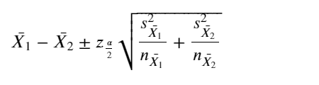
If the confidence interval contains 0, then there is 95% confidence that there is no difference in mean between the two variablles. The confidence interval of the variable in the training data can also be estimated. If the mean of the variable in the serving set falls outside this interval wecan flag that there is difference in means between the two variables.
The classical normal 95% confidence interval for the difference of the means assuming normal distrirution of the mean is:
import numpy as np
import pandas as pd
from scipy.stats import t
pd.set_option('display.max_columns', 30) # set so can see all columns of the DataFrame
import math
import numpy as np
from scipy.stats import norm
from scipy.stats import bootstrap
rng = np.random.default_rng()

m = train_df[numeric_cols].mean() - test_df[numeric_cols].mean()

me = 1.96* np.sqrt(train_df[numeric_cols].var()/train_df.shape[0] + test_df[numeric_cols].var()/test_df.shape[0])

res = pd.DataFrame({'Feature':numeric_cols,
                    'mean_ci_lower_limit': m- me,
                   'mean_ci_upper_limit': m+me,
                    'Train_mean':train_df[numeric_cols].mean(),'Test_mean':test_df[numeric_cols].mean()})
res
| Feature | mean_ci_lower_limit | mean_ci_upper_limit | Train_mean | Test_mean | |
|---|---|---|---|---|---|
| age | age | -1.491609 | 1.540420 | 51.856429 | 51.832023 |
| TSH | TSH | -1.810646 | 1.370124 | 4.562983 | 4.783244 |
| T3 | T3 | -0.088162 | 0.034031 | 2.011452 | 2.038517 |
| TT4 | TT4 | -1.482069 | 3.762244 | 109.640701 | 108.500613 |
| T4U | T4U | -0.007827 | 0.020980 | 1.001173 | 0.994596 |
| FTI | FTI | -2.270119 | 2.602522 | 110.870388 | 110.704187 |
Alternatively, the bootstrap confidence interval for the mean can be found as below by resampling with replacement. In bootstrap we create multiple resamples with replacement from the observed dataset. The commpute the effect size of interest(example difference in means) on each of these resamples. The bootstrap resamples of the effect size can then be used to determine the 95% Confidence Interval. The distribution of the mean of the resampled data approaches the normal distribution due to the central limit theorem even when the original distribution of the data is not normaly distributed. With the percentile method the suppose we have 1000 bootstrap samples and the sorted effect size from smallest to largest, the 25th and 975th effect size represents the 95% confidence interval.
- calculate difference in means on each of the 1000 bootstrap sample
- Sort the difference in mean in ascending order.
- Select the 2.5th percentile as the 25th value and the 97.5th percentile as the 975 value for the confidence interval.
%%time


num_iter = 10000
n_sample = train_df.shape[0]

boot_mean_train = np.zeros((num_iter, len(numeric_cols)))
boot_mean_test = np.zeros((num_iter, len(numeric_cols)))
#boot_var_train   =  np.zeros((num_iter, len(numeric_cols)))
#boot_var_test   =  np.zeros((num_iter, len(numeric_cols)))
boot_statistic   =  np.zeros((num_iter, len(numeric_cols)))
#boot_me   =  np.zeros((num_iter, len(numeric_cols)))

for i in range(num_iter):

    boot_mean_train[i,:]  = list(train_df[numeric_cols].sample(n=n_sample,replace=True).mean())
    boot_mean_test[i,:]  = list(test_df[numeric_cols].sample(n= n_sample,replace=True).mean())
    boot_statistic[i,:]   =  boot_mean_train[i,:] - boot_mean_test[i,:]


    #boot_var_train[i,:]  =  list(train_df[numeric_cols].sample(n= n_sample,replace=True).var())
    #boot_var_test[i,:]  =  list(test_df[numeric_cols].sample(n= n_sample,replace=True).var())
   # boot_me[i,:]  =  1.96* np.sqrt(boot_var_train[i,:]/train_df[numeric_cols].sample(n= n_sample,replace=True).shape[0] +
    #                               test_df[numeric_cols].var()/test_df[numeric_cols].sample(n= n_sample,replace=True).shape[0])


#normal method
#lower_interval = boot_statistic.mean(0)- 1.96*(boot_statistic.std(0)/np.sqrt(num_iter))
#upper_interval = boot_statistic.mean(0) + 1.96*(boot_statistic.std(0)/np.sqrt(num_iter))


# 95% CI using the  percentile method
lower_limit = np.sort(boot_statistic, axis=0)[25,:]
upper_limit = np.sort(boot_statistic, axis=0)[975,:]

#equivalently
lower_limit = np.quantile(boot_statistic, q=0.025,axis=0)
upper_limit = np.quantile(boot_statistic, q=0.975,axis=0)

res = pd.DataFrame({'Feature':numeric_cols,'LowerLimit':lower_limit,'UpperLimit':upper_limit,
                    'Train_mean':train_df[numeric_cols].mean(),'Test_mean':test_df[numeric_cols].mean()  })
res
CPU times: user 22.1 s, sys: 74.4 ms, total: 22.2 s
Wall time: 22.2 s
| Feature | LowerLimit | UpperLimit | Train_mean | Test_mean | |
|---|---|---|---|---|---|
| age | age | -1.471455 | 1.559323 | 51.856429 | 51.832023 |
| TSH | TSH | -1.905514 | 1.468802 | 4.562983 | 4.783244 |
| T3 | T3 | -0.096149 | 0.040580 | 2.011452 | 2.038517 |
| TT4 | TT4 | -1.583813 | 3.817105 | 109.640701 | 108.500613 |
| T4U | T4U | -0.008266 | 0.021863 | 1.001173 | 0.994596 |
| FTI | FTI | -2.493965 | 2.701709 | 110.870388 | 110.704187 |
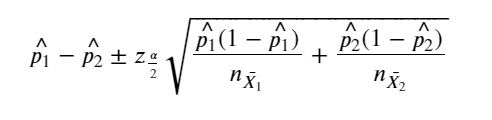
The classical 95% confidence interval for the difference in proportion for categorical variables with two levels can be found as below:
two_level_categorical = ['on thyroxine','query on thyroxine','on antithyroid medication',
             'sick','pregnant','thyroid surgery','I131 treatment','query hypothyroid',
             'query hyperthyroid','lithium','goitre','tumor','hypopituitary','psych',
             'TSH measured','T3 measured','TT4 measured','T4U measured']

n_sample = train_df.shape[0]


lower_limit = []
upper_limit  = []
p_test      = []
p_train  =   []
pdiff  = []
for column in two_level_categorical:
  dtest=pd.DataFrame(test_df[column].value_counts()/n_sample).reset_index().rename(columns={'index':'Value'})
  dtrain=pd.DataFrame(train_df[column].value_counts()/n_sample).reset_index().rename(columns={'index':'Value'})
  p1 = dtest.query('Value == "f"').iloc[0,1]
  p2 = dtrain.query('Value == "f"').iloc[0,1]
  margin_error = 1.96*np.sqrt((p1*(1-p1))/n_sample  + (p2*(1-p2))/n_sample)
  lower_limit.append((p1-p2) -margin_error)
  upper_limit.append((p1-p2) + margin_error)
  p_test.append(p1)
  p_train.append(p2)


res = pd.DataFrame({'Feature':two_level_categorical,'LowerLimit':lower_limit,'UpperLimit':upper_limit,
                    'Train_proportion':p_train,'Test_proportion':p_test  })
res
| Feature | LowerLimit | UpperLimit | Train_proportion | Test_proportion | |
|---|---|---|---|---|---|
| 0 | on thyroxine | -0.036739 | 0.011025 | 0.888571 | 0.875714 |
| 1 | query on thyroxine | -0.000214 | 0.017357 | 0.981429 | 0.990000 |
| 2 | on antithyroid medication | -0.008114 | 0.008114 | 0.987857 | 0.987857 |
| 3 | sick | -0.001527 | 0.027241 | 0.954286 | 0.967143 |
| 4 | pregnant | -0.008184 | 0.009613 | 0.985000 | 0.985714 |
| 5 | thyroid surgery | -0.010824 | 0.006539 | 0.987143 | 0.985000 |
| 6 | I131 treatment | -0.008187 | 0.011044 | 0.982143 | 0.983571 |
| 7 | query hypothyroid | -0.030910 | 0.003767 | 0.948571 | 0.935000 |
| 8 | query hyperthyroid | -0.029973 | 0.005688 | 0.944286 | 0.932143 |
| 9 | lithium | -0.003796 | 0.006654 | 0.994286 | 0.995714 |
| 10 | goitre | -0.004825 | 0.009111 | 0.990000 | 0.992143 |
| 11 | tumor | -0.005215 | 0.018072 | 0.971429 | 0.977857 |
| 12 | hypopituitary | -0.000685 | 0.002114 | 0.999286 | 1.000000 |
| 13 | psych | -0.008010 | 0.023724 | 0.947857 | 0.955714 |
| 14 | TSH measured | -0.006643 | 0.038071 | 0.093571 | 0.109286 |
| 15 | T3 measured | -0.027974 | 0.032260 | 0.207857 | 0.210000 |
| 16 | TT4 measured | -0.012640 | 0.024069 | 0.062857 | 0.068571 |
| 17 | T4U measured | -0.007805 | 0.037805 | 0.098571 | 0.113571 |
The bootstrap confidence interval for the proportion can also be found as shown below.It basicaly enatils obtaining the distribution of the diffeence i proportions by resampling with replacement then calcculating the 2.5th percentile as the lower confidence limit and 97.5th interval as the upper confidence limit.
two_level_categorical = ['on thyroxine','query on thyroxine','on antithyroid medication',
             'sick','pregnant','thyroid surgery','I131 treatment','query hypothyroid',
             'query hyperthyroid','lithium','goitre','tumor','hypopituitary','psych',
             'TSH measured','T3 measured','TT4 measured','T4U measured']


n_sample = train_df.shape[0]


num_iter = 1000
ptest2   =   np.zeros((len(two_level_categorical),1))
ptrain2   =   np.zeros((len(two_level_categorical),1))
ptrain_statistic   =  np.zeros((len(two_level_categorical), num_iter))
ptest_statistic   =   np.zeros((len(two_level_categorical), num_iter))
pdiff_statistic   =   np.zeros((len(two_level_categorical), num_iter))


for j in range(num_iter):
    for i,column in enumerate(two_level_categorical):
        dtest=pd.DataFrame(test_df[column].sample(n=n_sample,replace=True).value_counts()/n_sample).reset_index().rename(columns={'index':'Value'})
        dtrain=pd.DataFrame(train_df[column].sample(n=n_sample,replace=True).value_counts()/n_sample).reset_index().rename(columns={'index':'Value'})
        p1 = dtest.query('Value == "f"').iloc[0,1]
        p2 = dtrain.query('Value == "f"').iloc[0,1]
        ptrain2[i] =    p2
        ptest2[i] =     p1

    ptrain_statistic[:,j] =  ptrain2.flatten()
    ptest_statistic[:,j] =   ptest2.flatten()
    pdiff_statistic[:,j]  = ptrain2.flatten() - ptest2.flatten()
lower_limit  = np.sort(pdiff_statistic, axis=1)[:,25]
upper_limit  = np.sort(pdiff_statistic, axis=1)[:,975]

#equivalently
#lower_limit = np.quantile(pdiff_statistic, q=0.025,axis=1)
#upper_limit = np.quantile(boot_statistic, q=0.975,axis=1)


res = pd.DataFrame({'Feature':two_level_categorical,'LowerLimit':lower_limit,'UpperLimit':upper_limit,
                   'Train_proportion':p_train,'Test_proportion':p_test  })
res
| Feature | LowerLimit | UpperLimit | Train_proportion | Test_proportion | |
|---|---|---|---|---|---|
| 0 | on thyroxine | -0.012143 | 0.036429 | 0.888571 | 0.875714 |
| 1 | query on thyroxine | -0.017143 | -0.000714 | 0.981429 | 0.990000 |
| 2 | on antithyroid medication | -0.008571 | 0.007857 | 0.987857 | 0.987857 |
| 3 | sick | -0.027143 | 0.000714 | 0.954286 | 0.967143 |
| 4 | pregnant | -0.009286 | 0.007857 | 0.985000 | 0.985714 |
| 5 | thyroid surgery | -0.006429 | 0.011429 | 0.987143 | 0.985000 |
| 6 | I131 treatment | -0.010714 | 0.008571 | 0.982143 | 0.983571 |
| 7 | query hypothyroid | -0.003571 | 0.030714 | 0.948571 | 0.935000 |
| 8 | query hyperthyroid | -0.005000 | 0.029286 | 0.944286 | 0.932143 |
| 9 | lithium | -0.006429 | 0.003571 | 0.994286 | 0.995714 |
| 10 | goitre | -0.009286 | 0.005000 | 0.990000 | 0.992143 |
| 11 | tumor | -0.019286 | 0.005714 | 0.971429 | 0.977857 |
| 12 | hypopituitary | -0.002143 | 0.000000 | 0.999286 | 1.000000 |
| 13 | psych | -0.022857 | 0.008571 | 0.947857 | 0.955714 |
| 14 | TSH measured | -0.037143 | 0.007143 | 0.093571 | 0.109286 |
| 15 | T3 measured | -0.032143 | 0.028571 | 0.207857 | 0.210000 |
| 16 | TT4 measured | -0.025000 | 0.012857 | 0.062857 | 0.068571 |
| 17 | T4U measured | -0.039286 | 0.008571 | 0.098571 | 0.113571 |
Concept Drift Understanding
The severity of concept drift can be measured by using a dissimilarity metric to measure the difference between a new and previous concepts. The greater the quantified difference between the two distributions, the more severe the drift. Identifying the time a concept drift occurs and its duration is key to concept drift understanding.A drift is detected if the accuracy of a learning system drops below a predefined threshold. For data drift, if there is a statistically significant difference between two data samples. A drift detection threshold may be set at p-value to 95% or $2\sigma$ or a p-value of 99% or $3\sigma$. Data distribution-based drift detection algorithms report a drift alarm when two data samples have a statistically significant difference. The two sample test statistics used here include the Generalized Wilcoxon-test statistic.Concept drift understanding involves the drift detection start point, change period and end point. The difference between a benchmark accuracy of a model and the new degraded accuracy can be used as an indirect measure of the severity of drift. The severity of data drift can be measured by magnitude of the distance between the features in the two time frame.Kullback–Leibler divergence, \({\displaystyle D_{\text{KL}}(P\parallel Q)}{\displaystyle D_{\text{KL}}(P\parallel Q)}\) (also called relative entropy and I-divergence[1]) is measure of drift with value between \([0,1]\). 0 means the two distributions are the same and 1 means a new concept has occurred. The greater its value from 0, the more severe the drift is.
Drift Adaptation
There are three main techniques for adapting existing machine learning models to drift occurrence namely
- simple retraining
- ensemble retraining
- model adjusting.
For recurring concept drifts, an old model may be combined with a new one handle drift when it occurs. Examples of ensemble methods used here include Adaptive Random Forest (ARF) which extends RF with a concept drift detection algorithm ADWIN to make a decision when a degerading model should be replaced, Dynamic Weighted Majority(DWM). Models can be trained to adaptively learn from the changing data so that the model will be update itself.An example algorithm include online decision tree algorithm, called Very Fast Decision Tree classifier (VFDT)