Distributed Machine Learning with Spark ML
A host of Regression and classification models are available in Spark ML libary. The models include :
Classification
- Logistic regression(Binomial and Multinomial)
- Decision tree classifier
- Random forest classifier
- Gradient-boosted tree classifier
- Multilayer perceptron classifier
- Linear Support Vector Machine
- One-vs-Rest classifier (a.k.a. One-vs-All)
- Naive Bayes
Regression
- Linear regression
- Generalized linear regression
- Decision tree regression
- Random forest regression
- Gradient-boosted tree regression
- Survival regression
- Isotonic regression
- Random Forests
Load the rquired libraries below
import pyspark.sql.types as typ
from pyspark.sql.types import IntegerType
from pyspark.sql.functions import col
import findspark
import pyspark
from pyspark.sql.session import SparkSession
from pyspark.sql.types import *
from pyspark.ml import Pipeline
from pyspark.sql.functions import col
import pyspark.ml.feature as ft
import pyspark.ml.feature
from pyspark.ml import Pipeline
import pyspark.ml.evaluation as ev
from pyspark.ml import PipelineModel
from pyspark.ml import *
import pyspark.ml.tuning as tune
import pandas as pd
import os
import pyspark.sql.functions as F
from pyspark.sql.functions import *
from pyspark.sql.functions import col, when
import seaborn as sns; sns.set()
import matplotlib.pyplot as plt
from pyspark.ml.feature import OneHotEncoderEstimator, StringIndexer, VectorAssembler
from pyspark.ml.classification import LogisticRegression
import pyspark.ml.classification as cl
from pyspark.ml.feature import StandardScaler
from pyspark.ml.feature import IndexToString
Start a Spark session here. The command below starts a session and names it PySpark Machine Learning
spark = SparkSession\
        .builder\
        .appName("PySpark Machine Learning ")\
        .getOrCreate()
findspark.init()
path="/Anomalydetection/bank/"
Description of Data
The data is related with direct marketing campaigns of a Portuguese banking institution. The marketing campaigns were based on phone calls. Often, more than one contact to the same client was required, in order to access if the product (bank term deposit) would be (‘yes’) or not (‘no’) subscribed. The dataset consist of 45,211 observations with 16 attributes and an output attribute spanning from May 2008 to November 2010. The data is available on UCI machine learning repository
The classification goal is to predict if the client will subscribe (yes/no) a term deposit (variable y). Input variables:
bank client data: Attribute Information:
- age (numeric)
- job : type of job (categorical:”admin.”,”unknown”,”unemployed”,”management”,”housemaid”,”entrepreneur”,”student”,”blue-collar”,”self-employed”,”retired”,”technician”,”services”)
- marital : marital status (categorical: “married”,”divorced”,”single”; note: “divorced” means divorced or widowed)
- education (categorical: “unknown”,”secondary”,”primary”,”tertiary”)
- default: has credit in default? (binary: “yes”,”no”)
- balance: average yearly balance, in euros (numeric)
- housing: has housing loan? (binary: “yes”,”no”)
- loan: has personal loan? (binary: “yes”,”no”)
related with the last contact of the current campaign:
- contact: contact communication type (categorical: “unknown”,”telephone”,”cellular”)
- day: last contact day of the month (numeric)
- month: last contact month of year (categorical: “jan”, “feb”, “mar”, …, “nov”, “dec”)
- duration: last contact duration, in seconds (numeric)
other attributes:
- campaign: number of contacts performed during this campaign and for this client (numeric, includes last contact)
- pdays: number of days that passed by after the client was last contacted from a previous campaign (numeric, -1 means client was not previously contacted)
- previous: number of contacts performed before this campaign and for this client (numeric)
- poutcome: outcome of the previous marketing campaign (categorical: “unknown”,”other”,”failure”,”success”)
Output variable (desired target):
-
y - has the client subscribed a term deposit? (binary: “yes”,”no”)
-
Missing Attribute Values: None
d=pd.read_csv(os.path.join(path,'bank-full.csv'),sep=';')

#data = pd.read_csv(path+'bank-full.csv', sep=';')
#data.head()

d.columns


#d.info()


pd.unique(d['pdays'])
#d['pdays'].unique()

#numeric, -1 means client was not previously contacted,set it to 0
d.loc[d['pdays'] == -1, 'pdays']=0
#pd.unique(d['pdays'])

print(d.shape)

d.head()
(45211, 17)
| age | job | marital | education | default | balance | housing | loan | contact | day | month | duration | campaign | pdays | previous | poutcome | y | |
|---|---|---|---|---|---|---|---|---|---|---|---|---|---|---|---|---|---|
| 0 | 58 | management | married | tertiary | no | 2143 | yes | no | unknown | 5 | may | 261 | 1 | 0 | 0 | unknown | no |
| 1 | 44 | technician | single | secondary | no | 29 | yes | no | unknown | 5 | may | 151 | 1 | 0 | 0 | unknown | no |
| 2 | 33 | entrepreneur | married | secondary | no | 2 | yes | yes | unknown | 5 | may | 76 | 1 | 0 | 0 | unknown | no |
| 3 | 47 | blue-collar | married | unknown | no | 1506 | yes | no | unknown | 5 | may | 92 | 1 | 0 | 0 | unknown | no |
| 4 | 33 | unknown | single | unknown | no | 1 | no | no | unknown | 5 | may | 198 | 1 | 0 | 0 | unknown | no |
schema = StructType(
  [StructField('age', typ.IntegerType()),
    StructField('job', typ.StringType()),
    StructField('marital', typ.StringType()),
    StructField('education', typ.StringType()),
    StructField('default', typ.StringType()),
    StructField('balance', typ.IntegerType()),
    StructField('housing', typ.StringType()),
    StructField('loan', typ.StringType()),
    StructField('contact', typ.StringType()),
    StructField('day', typ.IntegerType()),
    StructField('month', typ.StringType()),
    StructField('duration', typ.IntegerType()),
    StructField('campaign', typ.IntegerType()),
    StructField('pdays', typ.IntegerType()),
    StructField('previous', typ.IntegerType()),
    StructField('poutcome', typ.StringType()),
    StructField('y', typ.StringType())
  ])
#df = spark.read.csv(os.path.join(path,'bank-full.csv'), sep=';', header=True,schema=schema)
df = spark.read.csv(os.path.join(path,'bank-full.csv'), sep=';', header = True, inferSchema = True)

#df = spark.read.options(header='true', inferschema='true', delimiter=';').csv(os.path.join(path,'bank-full.csv'))

df.cache()
df.show(5)
+---+------------+-------+---------+-------+-------+-------+----+-------+---+-----+--------+--------+-----+--------+--------+---+
|age|         job|marital|education|default|balance|housing|loan|contact|day|month|duration|campaign|pdays|previous|poutcome|  y|
+---+------------+-------+---------+-------+-------+-------+----+-------+---+-----+--------+--------+-----+--------+--------+---+
| 58|  management|married| tertiary|     no|   2143|    yes|  no|unknown|  5|  may|     261|       1|   -1|       0| unknown| no|
| 44|  technician| single|secondary|     no|     29|    yes|  no|unknown|  5|  may|     151|       1|   -1|       0| unknown| no|
| 33|entrepreneur|married|secondary|     no|      2|    yes| yes|unknown|  5|  may|      76|       1|   -1|       0| unknown| no|
| 47| blue-collar|married|  unknown|     no|   1506|    yes|  no|unknown|  5|  may|      92|       1|   -1|       0| unknown| no|
| 33|     unknown| single|  unknown|     no|      1|     no|  no|unknown|  5|  may|     198|       1|   -1|       0| unknown| no|
+---+------------+-------+---------+-------+-------+-------+----+-------+---+-----+--------+--------+-----+--------+--------+---+
only showing top 5 rows
df.printSchema()
root
 |-- age: integer (nullable = true)
 |-- job: string (nullable = true)
 |-- marital: string (nullable = true)
 |-- education: string (nullable = true)
 |-- default: string (nullable = true)
 |-- balance: integer (nullable = true)
 |-- housing: string (nullable = true)
 |-- loan: string (nullable = true)
 |-- contact: string (nullable = true)
 |-- day: integer (nullable = true)
 |-- month: string (nullable = true)
 |-- duration: integer (nullable = true)
 |-- campaign: integer (nullable = true)
 |-- pdays: integer (nullable = true)
 |-- previous: integer (nullable = true)
 |-- poutcome: string (nullable = true)
 |-- y: string (nullable = true)
Replace -1 in df.pdays with 0
df= df.withColumn("pdays", when(col("pdays") == -1,0).otherwise(col("pdays")))

df.select(['pdays']).show(2)
+-----+
|pdays|
+-----+
|    0|
|    0|
+-----+
only showing top 2 rows
#df.filter('pdays==-1').select(['pdays']).show(5)
df.describe().show()
+-------+------------------+-------+--------+---------+-------+------------------+-------+-----+--------+-----------------+-----+-----------------+------------------+------------------+------------------+--------+-----+
|summary|               age|    job| marital|education|default|           balance|housing| loan| contact|              day|month|         duration|          campaign|             pdays|          previous|poutcome|    y|
+-------+------------------+-------+--------+---------+-------+------------------+-------+-----+--------+-----------------+-----+-----------------+------------------+------------------+------------------+--------+-----+
|  count|             45211|  45211|   45211|    45211|  45211|             45211|  45211|45211|   45211|            45211|45211|            45211|             45211|             45211|             45211|   45211|45211|
|   mean| 40.93621021432837|   null|    null|     null|   null|1362.2720576850766|   null| null|    null|15.80641879188693| null|258.1630797814691| 2.763840658246887| 40.19782796222158|0.5803233726305546|    null| null|
| stddev|10.618762040975401|   null|    null|     null|   null|3044.7658291685243|   null| null|    null|8.322476153044589| null|257.5278122651712|3.0980208832791813|100.12874599059818|2.3034410449312164|    null| null|
|    min|                18| admin.|divorced|  primary|     no|             -8019|     no|   no|cellular|                1|  apr|                0|                 1|                -1|                 0| failure|   no|
|    max|                95|unknown|  single|  unknown|    yes|            102127|    yes|  yes| unknown|               31|  sep|             4918|                63|               871|               275| unknown|  yes|
+-------+------------------+-------+--------+---------+-------+------------------+-------+-----+--------+-----------------+-----+-----------------+------------------+------------------+------------------+--------+-----+
Summary statistics for numeric variables
numeric_features = [t[0] for t in df.dtypes if t[1] == 'int']
df.select(numeric_features).describe().toPandas().transpose()
| 0 | 1 | 2 | 3 | 4 | |
|---|---|---|---|---|---|
| summary | count | mean | stddev | min | max |
| age | 45211 | 40.93621021432837 | 10.618762040975401 | 18 | 95 |
| balance | 45211 | 1362.2720576850766 | 3044.7658291685243 | -8019 | 102127 |
| day | 45211 | 15.80641879188693 | 8.322476153044589 | 1 | 31 |
| duration | 45211 | 258.1630797814691 | 257.5278122651712 | 0 | 4918 |
| campaign | 45211 | 2.763840658246887 | 3.0980208832791813 | 1 | 63 |
| pdays | 45211 | 41.015195417044524 | 99.7926151457054 | 0 | 871 |
| previous | 45211 | 0.5803233726305546 | 2.3034410449312164 | 0 | 275 |
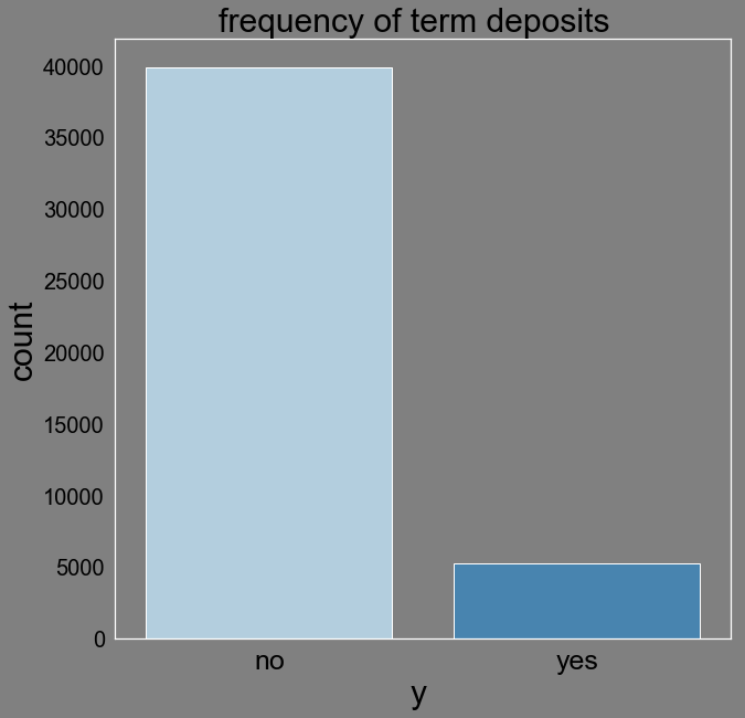
Count distinct values of deposit term(y). The clients with subscribed term deposits is about 88% compared with those without term deposits.
sum_y=df.select('y').count()
prop_y=df.select('y').groupby(df.y).count()

prop_y = prop_y \
    .withColumn('prop_y',
               (col('count')/sum_y)*100 \
                    )

prop_y.show()
#/45211
#.cast(typ.FloatType())
+---+-----+------------------+
|  y|count|            prop_y|
+---+-----+------------------+
| no|39922| 88.30151954170445|
|yes| 5289|11.698480458295547|
+---+-----+------------------+
bg_color = (0.5, 0.5, 0.5)

sns.set(rc={"font.style":"normal",
            "axes.facecolor":bg_color,
            "axes.titlesize":30,
            "figure.facecolor":bg_color,
            "text.color":"black",
            "xtick.color":"black",
            "ytick.color":"black",
            "axes.labelcolor":"black",
            "axes.grid":False,
            'axes.labelsize':30,
            'figure.figsize':(10.0, 10.0),
            'xtick.labelsize':25,
            'ytick.labelsize':20})

#plt.rcParams.update(params)
sns.countplot(d["y"],palette="Blues")
plt.xlabel('y ')
plt.title('frequency of term deposits  ')
plt.show()
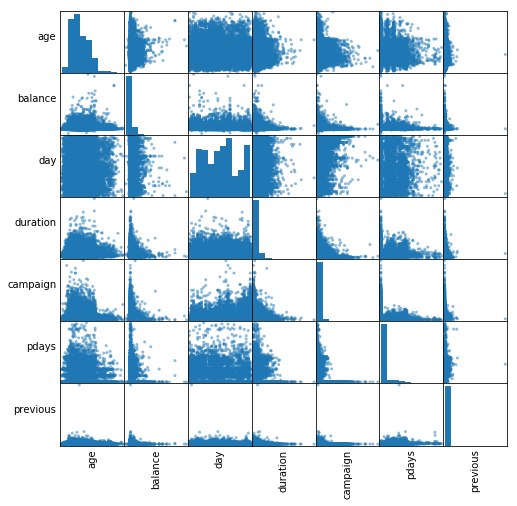
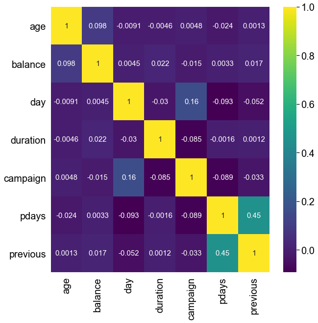
Correlations between independent variables.
numeric_data = df.select(numeric_features).toPandas()
axs = pd.plotting.scatter_matrix(numeric_data, figsize=(8, 8));
n = len(numeric_data.columns)
for i in range(n):
    v = axs[i, 0]
    v.yaxis.label.set_rotation(0)
    v.yaxis.label.set_ha('right')
    v.set_yticks(())
    h = axs[n-1, i]
    h.xaxis.label.set_rotation(90)
    h.set_xticks(())
corr = df.select(numeric_features).toPandas().corr()

sns.set(rc={"font.style":"normal",
            "axes.titlesize":30,
           "text.color":"black",
            "xtick.color":"black",
            "ytick.color":"black",
            "axes.labelcolor":"black",
            "axes.grid":False,
            'axes.labelsize':30,
            'figure.figsize':(10.0, 10.0),
            'xtick.labelsize':20,
            'ytick.labelsize':20})
sns.heatmap(corr,annot = True, annot_kws={"size": 15},cmap="viridis")

plt.show()
Preprocessing Data
The Spark ML library accepts only numeric input. We have some attributes that are categorical and others numeric. For the categorical features, first we convert to numeric categories with StringIndexer and then one-hot encode with the OneHotEncoderEstimator functions. The indexing introduces an implicit ordering among your categories, and is more suitable for ordinal variables (eg: low: 0, medium: 1, high: 2). The One-Hot encoding converts the categories into binary SparseVector. The pipeline will be used to tie the various feature transformations stages in preprocessing sringindexing, one-hot encoding and standardization
df.printSchema()
root
 |-- age: integer (nullable = true)
 |-- job: string (nullable = true)
 |-- marital: string (nullable = true)
 |-- education: string (nullable = true)
 |-- default: string (nullable = true)
 |-- balance: integer (nullable = true)
 |-- housing: string (nullable = true)
 |-- loan: string (nullable = true)
 |-- contact: string (nullable = true)
 |-- day: integer (nullable = true)
 |-- month: string (nullable = true)
 |-- duration: integer (nullable = true)
 |-- campaign: integer (nullable = true)
 |-- pdays: integer (nullable = true)
 |-- previous: integer (nullable = true)
 |-- poutcome: string (nullable = true)
 |-- y: string (nullable = true)
from pyspark.ml.feature import OneHotEncoderEstimator, StringIndexer, VectorAssembler


categoricalColumns = ['job','marital','education','default','housing','loan','contact','month','poutcome']
stages = []
for categoricalCol in categoricalColumns:
    # Category Indexing with StringIndexer
    stringIndexer = StringIndexer(inputCol = categoricalCol, outputCol = categoricalCol + 'Index')
    # Use OneHotEncoder to convert categorical variables into binary SparseVectors
    encoder = OneHotEncoderEstimator(inputCols=[stringIndexer.getOutputCol()], outputCols=[categoricalCol + "classVec"])
    stages += [stringIndexer, encoder]


labelIndexer = StringIndexer(inputCol = 'y', outputCol = 'label')


# Index labels, adding metadata to the label column.
# Fit on whole dataset to include all labels in index.
#labelIndexer = StringIndexer(inputCol="y", outputCol="label")
#labels = labelIndexer.fit(df).labels


stages += [labelIndexer]

numericCols = ["day","age", "balance", "duration", "campaign", "pdays","previous"]
assemblerInputs = [c + "classVec" for c in categoricalColumns] + numericCols
assembler = VectorAssembler(inputCols=assemblerInputs, outputCol="unscaled_features")
stages += [assembler]


#standardize and scale features to mean 0 and variance 1
standardScaler = StandardScaler(inputCol="unscaled_features",
                                outputCol="features",
                                withMean=True,
                                withStd=True)
stages += [standardScaler]


# Convert indexed labels back to original labels.
#labelConverter = IndexToString(inputCol="prediction", outputCol="predictedLabel", labels=labels)
from pyspark.ml import Pipeline


pipeline = Pipeline(stages = stages)
pipelineModel = pipeline.fit(df)
dff = pipelineModel.transform(df)
The VectorAssembler above combines all the feature columns(numeric, one-hot encoded binary vector and normalizer ) into a single vector column. The Pipeline puts the data through all of the feature transformations we described in a single call. We use the StringIndexer again to encode our labels to label indices.
pd.DataFrame(dff.take(4), columns=dff.columns).transpose()
| 0 | 1 | 2 | 3 | |
|---|---|---|---|---|
| age | 58 | 44 | 33 | 47 |
| job | management | technician | entrepreneur | blue-collar |
| marital | married | single | married | married |
| education | tertiary | secondary | secondary | unknown |
| default | no | no | no | no |
| balance | 2143 | 29 | 2 | 1506 |
| housing | yes | yes | yes | yes |
| loan | no | no | yes | no |
| contact | unknown | unknown | unknown | unknown |
| day | 5 | 5 | 5 | 5 |
| month | may | may | may | may |
| duration | 261 | 151 | 76 | 92 |
| campaign | 1 | 1 | 1 | 1 |
| pdays | 0 | 0 | 0 | 0 |
| previous | 0 | 0 | 0 | 0 |
| poutcome | unknown | unknown | unknown | unknown |
| y | no | no | no | no |
| jobIndex | 1 | 2 | 7 | 0 |
| jobclassVec | (0.0, 1.0, 0.0, 0.0, 0.0, 0.0, 0.0, 0.0, 0.0, ... | (0.0, 0.0, 1.0, 0.0, 0.0, 0.0, 0.0, 0.0, 0.0, ... | (0.0, 0.0, 0.0, 0.0, 0.0, 0.0, 0.0, 1.0, 0.0, ... | (1.0, 0.0, 0.0, 0.0, 0.0, 0.0, 0.0, 0.0, 0.0, ... |
| maritalIndex | 0 | 1 | 0 | 0 |
| maritalclassVec | (1.0, 0.0) | (0.0, 1.0) | (1.0, 0.0) | (1.0, 0.0) |
| educationIndex | 1 | 0 | 0 | 3 |
| educationclassVec | (0.0, 1.0, 0.0) | (1.0, 0.0, 0.0) | (1.0, 0.0, 0.0) | (0.0, 0.0, 0.0) |
| defaultIndex | 0 | 0 | 0 | 0 |
| defaultclassVec | (1.0) | (1.0) | (1.0) | (1.0) |
| housingIndex | 0 | 0 | 0 | 0 |
| housingclassVec | (1.0) | (1.0) | (1.0) | (1.0) |
| loanIndex | 0 | 0 | 1 | 0 |
| loanclassVec | (1.0) | (1.0) | (0.0) | (1.0) |
| contactIndex | 1 | 1 | 1 | 1 |
| contactclassVec | (0.0, 1.0) | (0.0, 1.0) | (0.0, 1.0) | (0.0, 1.0) |
| monthIndex | 0 | 0 | 0 | 0 |
| monthclassVec | (1.0, 0.0, 0.0, 0.0, 0.0, 0.0, 0.0, 0.0, 0.0, ... | (1.0, 0.0, 0.0, 0.0, 0.0, 0.0, 0.0, 0.0, 0.0, ... | (1.0, 0.0, 0.0, 0.0, 0.0, 0.0, 0.0, 0.0, 0.0, ... | (1.0, 0.0, 0.0, 0.0, 0.0, 0.0, 0.0, 0.0, 0.0, ... |
| poutcomeIndex | 0 | 0 | 0 | 0 |
| poutcomeclassVec | (1.0, 0.0, 0.0) | (1.0, 0.0, 0.0) | (1.0, 0.0, 0.0) | (1.0, 0.0, 0.0) |
| label | 0 | 0 | 0 | 0 |
| unscaled_features | (0.0, 1.0, 0.0, 0.0, 0.0, 0.0, 0.0, 0.0, 0.0, ... | (0.0, 0.0, 1.0, 0.0, 0.0, 0.0, 0.0, 0.0, 0.0, ... | (0.0, 0.0, 0.0, 0.0, 0.0, 0.0, 0.0, 1.0, 0.0, ... | (1.0, 0.0, 0.0, 0.0, 0.0, 0.0, 0.0, 0.0, 0.0, ... |
| features | [-0.5237337507789468, 1.9442485627526624, -0.4... | [-0.5237337507789468, -0.5143261518338231, 2.2... | [-0.5237337507789468, -0.5143261518338231, -0.... | [1.909324881204917, -0.5143261518338231, -0.44... |
### Randomly split data into training and test sets. set seed for reproducibility
(training, test) = dff.randomSplit([0.7, 0.3], seed=1)

print('Training Dataset Count: {}'.format(training.count()))
print('Training Dataset Count: {}'.format(test.count()))
Training Dataset Count: 31745
Training Dataset Count: 13466
Logistic Regression Model
Logistic regression is a statistical method to predict a categorical response. It is a special case of Generalized Linear models that predicts the probability of the outcomes. In spark.ml logistic regression can be used to predict a binary outcome by using binomial logistic regression, or it can be used to predict a multiclass outcome by using multinomial logistic regression.
Multinomial logistic regression can be used for binary classification by setting the family param to “multinomial”. It will produce two sets of coefficients and two intercepts.
The parameters in the logistic regression model also include maxIter, regParam and elasticNetParam. The model could be used to perform Elastic-Net Regularization with Logistic Regression, LASSO or ridge logistic regression. elasticNetParam corresponds to α and regParam corresponds to λ.
from pyspark.ml.classification import LogisticRegression

# Create initial LogisticRegression model
lr = LogisticRegression(labelCol="label", featuresCol="features", maxIter=10)

# Train model with Training Data
lrModel = lr.fit(training)
Make predictions on the test set.
# Make predictions on test data using the transform() method.
# LogisticRegression.transform() will only use the 'features' column.
predictions = lrModel.transform(test)

predictions.select( 'label', 'rawPrediction', 'prediction', 'probability').show(10)
+-----+--------------------+----------+--------------------+
|label|       rawPrediction|prediction|         probability|
+-----+--------------------+----------+--------------------+
|  0.0|[1.63721316342582...|       0.0|[0.83715537531275...|
|  0.0|[1.57206439631216...|       0.0|[0.82807770516930...|
|  1.0|[1.38086487179207...|       0.0|[0.79912986653101...|
|  0.0|[2.33406801174141...|       0.0|[0.91165950908026...|
|  0.0|[1.78185980781216...|       0.0|[0.85592636260920...|
|  1.0|[1.14313230786505...|       0.0|[0.75825427022485...|
|  1.0|[1.93349111401764...|       0.0|[0.87363533012628...|
|  0.0|[2.47630882446761...|       0.0|[0.92246420157909...|
|  1.0|[0.53740310620167...|       0.0|[0.63120810753530...|
|  0.0|[0.75876231413912...|       0.0|[0.68108495849814...|
+-----+--------------------+----------+--------------------+
only showing top 10 rows
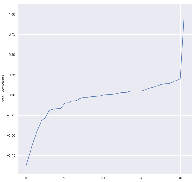
We can obtain the coefficients by using LogisticRegressionModel’s attributes.
import matplotlib.pyplot as plt
import numpy as np
beta = np.sort(lrModel.coefficients)
plt.plot(beta)
plt.ylabel('Beta Coefficients')
plt.show()
Summarize the model over the training set, we can also obtain the receiver-operating characteristic and areaUnderROC.
trainingSummary = lrModel.summary
roc = trainingSummary.roc.toPandas()
plt.plot(roc['FPR'],roc['TPR'])
plt.ylabel('False Positive Rate')
plt.xlabel('True Positive Rate')
plt.title('ROC Curve')
plt.show()
print('Training Dataset AUC: {}'.format(trainingSummary.areaUnderROC))
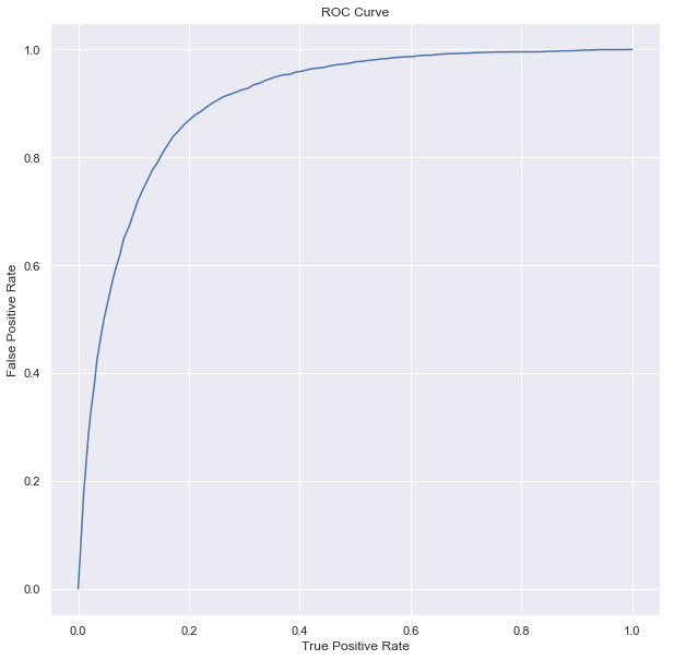
Training Dataset AUC: 0.9045120993163305
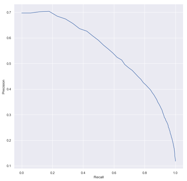
Precision and recall.
# Import numpy, pandas, and ggplot
import numpy as np
from pandas import *
#from ggplot import *
#from pandas.lib import Timestamp
#from pandas import Timestamp

# Create scatter plot and two regression models (scaling exponential) using ggplot
#p = ggplot(pr, aes('recall','precision')) + geom_line()
    #geom_point(color='blue') +
    #geom_line(pydf, color='red')
    #geom_line(pydf, aes('pop','predB'), color='green')
    #scale_x_log10() + scale_y_log10()
#p
pr = trainingSummary.pr.toPandas()
plt.plot(pr['recall'],pr['precision'])
plt.ylabel('Precision')
plt.xlabel('Recall')
plt.show()
Evaluate our Logistic Regression model.
We can use BinaryClassificationEvaluator to evaluate our model. We can set the required column names in rawPredictionCol and labelCol Param and the metric in metricName Param.
from pyspark.ml.evaluation import BinaryClassificationEvaluator
evaluator = BinaryClassificationEvaluator()

print('Logistic Model Test Area Under ROC: {}'.format(evaluator.evaluate(predictions)))
Test Area Under ROC: 0.9123415253544724
Random Forest
Random forests are ensembles of decision trees that improves accuracy. Random forests combine many decision trees in order to reduce the risk of overfitting.
The Spark ML library implementation supports random forests for binary and multiclass classification and for regression, using both continuous and categorical features.
from pyspark.ml.classification import RandomForestClassifier

# Create an initial RandomForest model.
rf = RandomForestClassifier(labelCol="label", featuresCol="features")

# Train model with Training Data
rfModel = rf.fit(training)
Let’s now create a single column with all the features collated together.
# Make predictions on test data using the Transformer.transform() method.
predictions = rfModel.transform(test)
# View model's predictions and probabilities of each prediction class
selected = predictions.select("label", "prediction", "probability")
selected.show(10)
+-----+----------+--------------------+
|label|prediction|         probability|
+-----+----------+--------------------+
|  0.0|       0.0|[0.88811261811572...|
|  0.0|       0.0|[0.87160035839545...|
|  1.0|       0.0|[0.86229855134246...|
|  0.0|       0.0|[0.88865524599928...|
|  0.0|       0.0|[0.89654402678231...|
|  1.0|       0.0|[0.85324123871973...|
|  1.0|       0.0|[0.88817420681755...|
|  0.0|       0.0|[0.90258386549908...|
|  1.0|       0.0|[0.85921128927556...|
|  0.0|       0.0|[0.88657306773581...|
+-----+----------+--------------------+
only showing top 10 rows
We can evaluate the Random Forest model with BinaryClassificationEvaluator.
from pyspark.ml.evaluation import BinaryClassificationEvaluator


evaluator = BinaryClassificationEvaluator()
evaluator.evaluate(predictions)

print('RF Model Test Area Under ROC: {}'.format(evaluator.evaluate(predictions)))
Test Area Under ROC: 0.8877592443645499
Saving the model
PySpark allows you to save the Pipeline definition for later use.
from pyspark.mllib.classification import LogisticRegressionWithLBFGS, LogisticRegressionModel

pipelinePath = '/Logistic_Pipeline'
pipelineModel.write().overwrite().save(pipelinePath)

#loadedPipelineModel = PipelineModel.load(modelPath)

#pipelineModel = loadedPipelineModel.fit(df)
#pipelineModel.save("/path")
The pipeline can be loaded and used straight away to .fit(…) and predict.
You can also save the whole model
modelPath = './infant_oneHotEncoder_Logistic_PipelineModel'
lrModel.write().overwrite().save(modelPath)

#loadedPipelineModel = PipelineModel.load(modelPath)
#test_loadedModel = loadedPipelineModel.transform(test)
Gradient-Boosted Tree Classifier
Gradient-Boosted Trees like random forest are also ensembles of decision trees.The Boosting algorithm iteratively train decision trees in order to minimize a loss function. The Spark ML implementation supports Gradient-Boosting for binary and multiclass classification and for regression, using both continuous and categorical features.
from pyspark.ml.classification import GBTClassifier

gbt = GBTClassifier(labelCol="label", featuresCol="features",maxIter=10)


# Chain indexers and GBT in a Pipeline
pipeline = Pipeline(stages=stages+[gbt])

### Randomly split data into training and test sets. set seed for reproducibility
(traininggbt, testgbt) = df.randomSplit([0.7, 0.3], seed=1)


# Train model.  This also runs the indexers.
gbtModel = pipeline.fit(traininggbt)

# Make predictions.
predictions =gbtModel.transform(testgbt)

# Select example rows to display.
predictions.select('label', 'prediction', 'probability').show(10)
+-----+----------+--------------------+
|label|prediction|         probability|
+-----+----------+--------------------+
|  0.0|       0.0|[0.81156118162434...|
|  0.0|       0.0|[0.79678515589243...|
|  1.0|       0.0|[0.70971584038432...|
|  0.0|       0.0|[0.89625862589373...|
|  0.0|       0.0|[0.85447621277148...|
|  1.0|       0.0|[0.82249890660556...|
|  1.0|       0.0|[0.87178030239148...|
|  0.0|       0.0|[0.89625862589373...|
|  1.0|       0.0|[0.72065322437528...|
|  0.0|       0.0|[0.81156118162434...|
+-----+----------+--------------------+
only showing top 10 rows
Evaluate our Gradient-Boosted Tree Classifier.
evaluator = BinaryClassificationEvaluator()
print("GBT Test Area Under ROC: " + str(evaluator.evaluate(predictions, {evaluator.metricName: "areaUnderROC"})))
Test Area Under ROC: 0.9163605060149584
Parameter hyper-tuning : Grid search
We can specify the list of parameters we want our model to loop through using ParamGridBuilder and the CrossValidator.
For these specified values, 3 values for maxDepth, 2 values for maxBin, and 2 values for numTrees, this grid will have 3 x 2 x 2 = 12 parameter settings for CrossValidator to choose from. We will create a 5-fold CrossValidator.
Random Forest
# Create ParamGrid for Cross Validation
from pyspark.ml.tuning import ParamGridBuilder, CrossValidator

paramGrid = (ParamGridBuilder()
             .addGrid(rf.maxDepth, [2, 4, 6])
             .addGrid(rf.maxBins, [20, 60])
             .addGrid(rf.numTrees, [5, 20])
             .build())

# Create 5-fold CrossValidator
cv = CrossValidator(estimator=rf, estimatorParamMaps=paramGrid,
                    evaluator=evaluator, numFolds=5)

# Run cross validations.  This can take about 6 minutes since it is training over 20 trees!
cvModel = cv.fit(training)
bestModel = cvModel.bestModel
# Generate predictions for the test set
finalPredictions = bestModel.transform(training)
# Evaluate best model

print('RF Model Test Area Under ROC: {}'.format(evaluator.evaluate(finalPredictions)))

# View Best model's predictions and probabilities of each prediction class
selected = predictions.select("label", "prediction", "probability")
selected.show(10)
0.9041133836611712
+-----+----------+--------------------+
|label|prediction|         probability|
+-----+----------+--------------------+
|  0.0|       0.0|[0.81156118162434...|
|  0.0|       0.0|[0.79678515589243...|
|  1.0|       0.0|[0.70971584038432...|
|  0.0|       0.0|[0.89625862589373...|
|  0.0|       0.0|[0.85447621277148...|
|  1.0|       0.0|[0.82249890660556...|
|  1.0|       0.0|[0.87178030239148...|
|  0.0|       0.0|[0.89625862589373...|
|  1.0|       0.0|[0.72065322437528...|
|  0.0|       0.0|[0.81156118162434...|
+-----+----------+--------------------+
only showing top 10 rows
Hyper-parameter tuning improves the accuracy of the random forest model from 0.88775 to 0.90411
Logistic Regression Model
An elastic net logistic regression with the parameters specified below :
from pyspark.ml.tuning import ParamGridBuilder, CrossValidator

# Create ParamGrid for Cross Validation
paramGrid = (ParamGridBuilder()
             .addGrid(lr.regParam, [0.01, 0.5, 0.9])
             .addGrid(lr.elasticNetParam, [0.0, 0.5, 1.0])
             .addGrid(lr.maxIter, [1, 5, 10])
             .build())

# Create 5-fold CrossValidator
cv = CrossValidator(estimator=lr, estimatorParamMaps=paramGrid,
                    evaluator=evaluator, numFolds=5)

# Run cross validations
cvModel = cv.fit(training)

# Use test set to measure the accuracy of our model on new data
predictions = cvModel.transform(test)
# cvModel uses the best model found from the Cross Validation
# Evaluate best model

print('Logistic Model Test Area Under ROC: {}'.format(evaluator.evaluate(predictions)))
0.9117952439594329
#We can also access the model's feature weights and intercepts easily

print('Model Intercept: ', cvModel.bestModel.intercept)

weights = cvModel.bestModel.coefficients
weights = [(float(w),) for w in weights]  # convert numpy type to float, and to tuple
weightsDF = spark.createDataFrame(weights, ["Feature Weight/regression Coefficients"])
weightsDF.show(5)

# View best model's predictions and probabilities of each prediction class
selected = predictions.select("label", "prediction", "probability")
selected.show(5)
Model Intercept:  -2.6309197104114284
+--------------------------------------+
|Feature Weight/regression Coefficients|
+--------------------------------------+
|                  -0.07073005694401832|
|                  0.001887728412912...|
|                  2.371519730171667...|
|                    0.0435185686230492|
|                  -0.01651731260686...|
+--------------------------------------+
only showing top 5 rows

+-----+----------+--------------------+
|label|prediction|         probability|
+-----+----------+--------------------+
|  0.0|       0.0|[0.83136792427306...|
|  0.0|       0.0|[0.83403384899106...|
|  1.0|       0.0|[0.77640736063075...|
|  0.0|       0.0|[0.89840924140505...|
|  0.0|       0.0|[0.87557287412278...|
+-----+----------+--------------------+
only showing top 5 rows
The cvModel will return the best model estimated. The parameters for the best model can be obtained as shown below :
results = [
    (
        [
            {key.name: paramValue}
            for key, paramValue
            in zip(
                params.keys(),
                params.values())
        ], metric
    )
    for params, metric
    in zip(
        cvModel.getEstimatorParamMaps(),
        cvModel.avgMetrics
    )
]

sorted(results,
       key=lambda el: el[1],
       reverse=True)[0]
([{'regParam': 0.01}, {'elasticNetParam': 0.0}, {'maxIter': 10}],
 0.90294114115149)
Train-Validation splitting
Use the ChiSqSelector to select only top 5 features, thus limiting the complexity of our model.
import pyspark.ml.tuning as tune
import pyspark.ml.classification as cl
from pyspark.ml.tuning import ParamGridBuilder, TrainValidationSplit


# We use a ParamGridBuilder to construct a grid of parameters to search over.
# TrainValidationSplit will try all combinations of values and determine best model using
# the evaluator.
paramGrid = ParamGridBuilder()\
    .addGrid(lr.regParam, [0.1, 0.01]) \
    .addGrid(lr.fitIntercept, [False, True])\
    .addGrid(lr.elasticNetParam, [0.0, 0.5, 1.0])\
    .build()

# In this case the estimator is simply the linear regression.
# A TrainValidationSplit requires an Estimator, a set of Estimator ParamMaps, and an Evaluator.
tvs = TrainValidationSplit(estimator=lr,
                           estimatorParamMaps=paramGrid,
                           evaluator=evaluator,
                           # 80% of the data will be used for training, 20% for validation.
                           trainRatio=0.8)

# Run TrainValidationSplit, and choose the best set of parameters.
tvsModel = tvs.fit(training)
The TrainValidationSplit object gets created in the same fashion as the CrossValidator model.
results = tvsModel.transform(test)


print('Logistic Model Test Area Under ROC: {}'.format(evaluator.evaluate(results,
     {evaluator.metricName: 'areaUnderROC'})))

print('Logistic Model Test Area Under PR: {}'.format(evaluator.evaluate(results,
     {evaluator.metricName: 'areaUnderPR'})))

# Make predictions on test data. model is the model with combination of parameters
# that performed best.
tvsModel.transform(test)\
    .select("probability", "label", "prediction")\
    .show(5)
Logistic Model Test Area Under ROC: 0.910786510492865
Logistic Model Test Area Under PR: 0.5632996614786637
+--------------------+-----+----------+
|         probability|label|prediction|
+--------------------+-----+----------+
|[0.41065007831036...|  0.0|       1.0|
|[0.42145041212388...|  0.0|       1.0|
|[0.38639008875536...|  1.0|       1.0|
|[0.47401249269605...|  0.0|       1.0|
|[0.51132340556245...|  0.0|       0.0|
+--------------------+-----+----------+
only showing top 5 rows
print(spark.version)
#end spark session
spark.stop()