Introduction
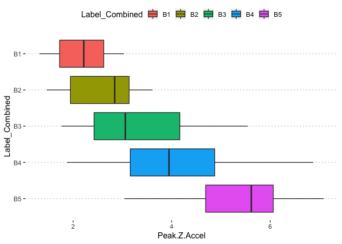
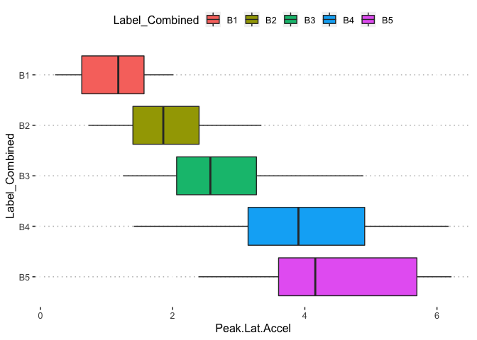
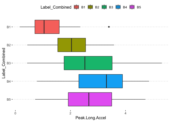
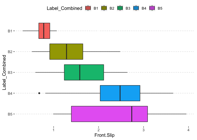
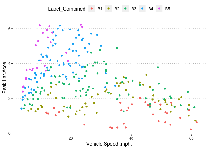
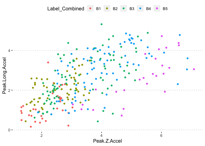
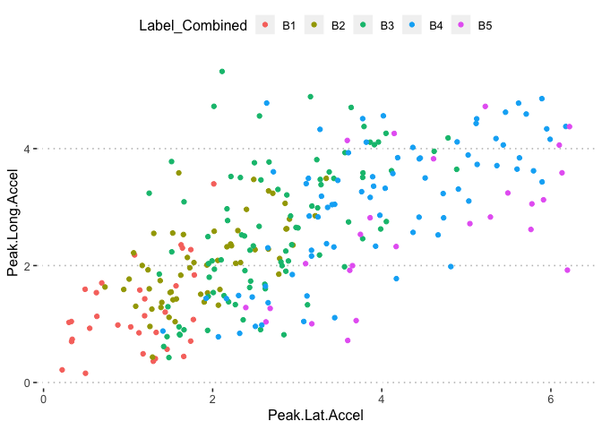
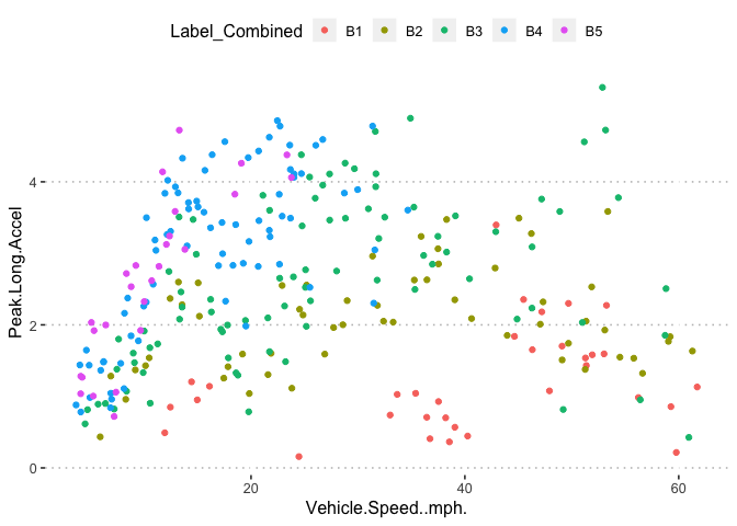
Our goal is to predict the depth and size of a pothole based on features collecting by vehicle running over potholes such as vehicle speed,acceleration ,direction ect. The number of distinct labels Label_Combined B1,..B5 represents various increasing size and depth of potholes.
Load Required Packages
The pacman package provides a convenient way to load packages. It installs the package before loading if it not already installed.One of my favorite themes that I use with ggplot is the theme_pubclean. Here I set all themes with ggplot by it.
rm(list=ls())

#set.seed(4)
set.seed(7)


pacman::p_load(tidyverse,janitor,DataExplorer,skimr,ggpubr,viridis,kableExtra,caret,lightgbm,recipes,rsample,yardstick,pROC,xgboost,doParallel,mlr,readxl,stringr,parallel,VIM,GGally,DALEX,MLmetrics)


#Load  variable importance plot
source("Varplot.R")

source("EvaluationMetrics.R")


theme_set(theme_pubclean())
Equivalently the rio package provides a unified approach to importing a variety of file formats into R. The date variable is not in a standard date format so we convert to a standard format thus separating year, month and day by ‘-‘. We can take a look at the first few rows of the data afterwards. The str_c function from the stringr package works similarly to the paste function
potholedata<- rio::import("/POTHOLEDETECTION/pothole.xlsx",sheet="Sheet6")

potholedata<-potholedata%>%mutate_if(is.character,as_factor)%>%rename(Label_Combined=Feature,Label=Feature2)


Date=paste(substr(20180709, 1, 4),substr(20180709, 5, 6),substr(20180709, 7, 8),sep = "-")

#Equivalently
Date<-str_c(substr(20180709, 1, 4),"-",substr(20180709, 5, 6),"-",substr(20180709, 7, 8))

extracdate<-function(x){
d<-str_c(str_sub(x, 1, 4),str_sub(x, 5, 6),str_sub(x, 7, 8),sep = "-")
 return(d)
}


potholedata$Date<-as.Date(as_vector(purrr::map(potholedata$Date,extracdate)) )


#sapply(potholedata$Date, extracdate)


potholedata%>%head()%>%
  kable(escape = F, align = "c") %>%
  kable_styling(c("striped", "condensed"), full_width = F)
| Label_Combined | Label | Peak.Duration | Vehicle.Speed..mph. | Peak.Z.Accel | Peak.Lat.Accel | Peak.Long.Accel | Front.Slip | Right.Slip | Left.Slip | Direction | MLT1.Feature | MLT2.Feature | File | Date |
|---|---|---|---|---|---|---|---|---|---|---|---|---|---|---|
| B1 | P1 | 0.544 | 11.93148 | 1.327386 | 1.1773803 | 0.4910319 | 0.4385430 | 0.1112423 | 0.3469242 | Left3 | Type1 | N/A | Cal_EL1000Avg_1014 | 2018-07-09 |
| B1 | P1 | 0.534 | 12.45331 | 1.335112 | 1.1289830 | 0.8495341 | 0.5327276 | 0.1025403 | 0.4539765 | Left1 | Type1 | N/A | Cal_EL1000Avg_1014 | 2018-07-09 |
| B1 | P1 | 0.470 | 14.43407 | 1.383979 | 1.4389222 | 1.2037202 | 0.7060992 | 0.1216020 | 0.6253896 | Left1 | Type1 | N/A | Cal_EL1000Avg_1014 | 2018-07-09 |
| B1 | P1 | 0.464 | 14.97096 | 1.317055 | 1.0312775 | 0.9508938 | 0.7458671 | 0.1410580 | 0.7275356 | Left1 | Type1 | N/A | Cal_EL1000Avg_1519 | 2018-07-09 |
| B1 | P1 | 0.416 | 16.11388 | 1.325739 | 1.1956568 | 1.1412229 | 0.5629772 | 0.1215295 | 0.3926258 | Left3 | Type1 | N/A | Cal_EL1000Avg_1519 | 2018-07-09 |
| B1 | P1 | 0.184 | 24.47751 | 1.639389 | 0.4963087 | 0.1579519 | 0.3131939 | 0.1071209 | 0.4625270 | Left3 | Hump | Crest | Cal_EL1000Avg_2024 | 2018-07-09 |
Exploratory Data Analysis
We can take a pictorial look at the variables in the dataset courtesy the plot_str from the DataExplorer package.Alternatively the glimpse function in tidyverse can also be used to inspect the variables.
plot_str(potholedata)

glimpse(potholedata)
## Observations: 280
## Variables: 15
## $ Label_Combined      <fct> B1, B1, B1, B1, B1, B1, B1, B1, B1, B1, B1...
## $ Label               <fct> P1, P1, P1, P1, P1, P1, P1, P1, P1, P1, P1...
## $ Peak.Duration       <dbl> 0.544, 0.534, 0.470, 0.464, 0.416, 0.184, ...
## $ Vehicle.Speed..mph. <dbl> 11.93148, 12.45331, 14.43408, 14.97096, 16...
## $ Peak.Z.Accel        <dbl> 1.327386, 1.335112, 1.383979, 1.317055, 1....
## $ Peak.Lat.Accel      <dbl> 1.1773803, 1.1289830, 1.4389222, 1.0312775...
## $ Peak.Long.Accel     <dbl> 0.4910319, 0.8495341, 1.2037202, 0.9508938...
## $ Front.Slip          <dbl> 0.4385430, 0.5327276, 0.7060992, 0.7458671...
## $ Right.Slip          <dbl> 0.11124231, 0.10254033, 0.12160195, 0.1410...
## $ Left.Slip           <dbl> 0.3469242, 0.4539765, 0.6253896, 0.7275356...
## $ Direction           <fct> Left3, Left1, Left1, Left1, Left3, Left3, ...
## $ MLT1.Feature        <fct> Type1, Type1, Type1, Type1, Type1, Hump, T...
## $ MLT2.Feature        <fct> N/A, N/A, N/A, N/A, N/A, Crest, N/A, N/A, ...
## $ File                <fct> Cal_EL1000Avg_1014, Cal_EL1000Avg_1014, Ca...
## $ Date                <date> 2018-07-09, 2018-07-09, 2018-07-09, 2018-...
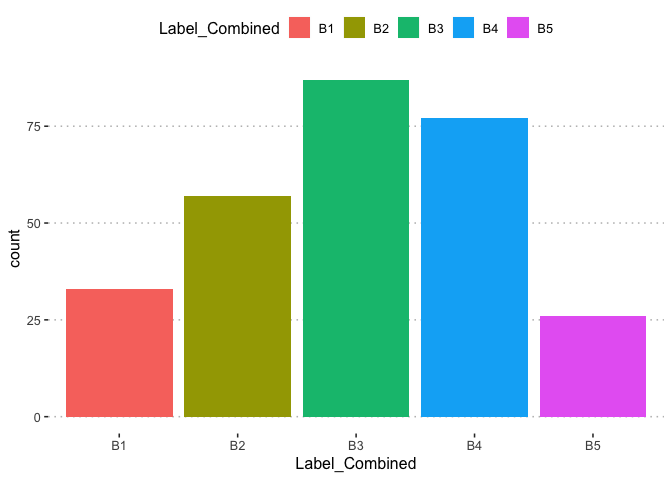
The labels distribution is not severely imbalanced to create concern in evaluation of the models which shall be built later.
table(potholedata$Label)
##
## P1 P2 P3 P4 P5 P6 P7 P8 P9
## 33 57 55 32 33 22 22 13 13
#check classes distribution
prop.table(table(potholedata$Label))*100
##
##        P1        P2        P3        P4        P5        P6        P7
## 11.785714 20.357143 19.642857 11.428571 11.785714  7.857143  7.857143
##        P8        P9
##  4.642857  4.642857
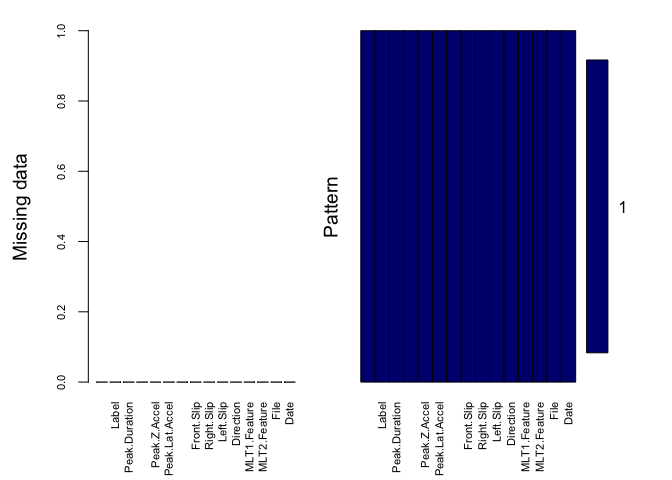
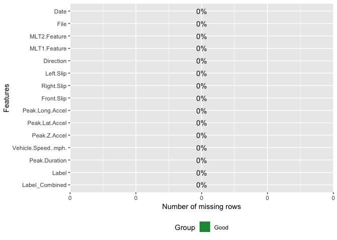
There are no missing observations in the data. Handling missing data in machine learning is very important. Several ways of dealing with missing values include mean and median imputation for continous and catergorical variables respectively. Several supervised learning algorthms such as random forest are also commonly used to impute missing values. Missing value imputation is a topic that would be looked at in depth later on.
aggr(potholedata , col=c('navyblue','yellow'),
                    numbers=TRUE, sortVars=TRUE,
                    labels=names(potholedata), cex.axis=.7,
                    gap=3, ylab=c("Missing data","Pattern"))
##
##  Variables sorted by number of missings:
##             Variable Count
##       Label_Combined     0
##                Label     0
##        Peak.Duration     0
##  Vehicle.Speed..mph.     0
##         Peak.Z.Accel     0
##       Peak.Lat.Accel     0
##      Peak.Long.Accel     0
##           Front.Slip     0
##           Right.Slip     0
##            Left.Slip     0
##            Direction     0
##         MLT1.Feature     0
##         MLT2.Feature     0
##                 File     0
##                 Date     0
plot_missing(potholedata)
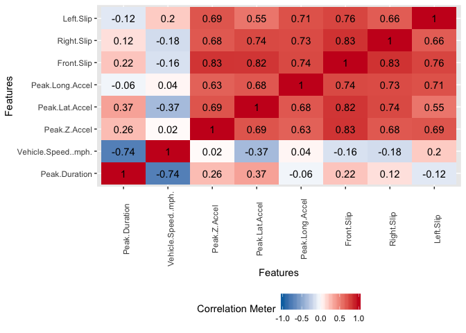
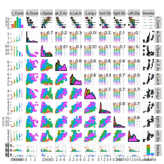
There exist significant correlation between some of the variables. This is not suprising because some of the features were engineered from others already present.
plot_correlation(potholedata,type = "continuous",theme_config = list(legend.position = "bottom", axis.text.x =
  element_text(angle = 90)))
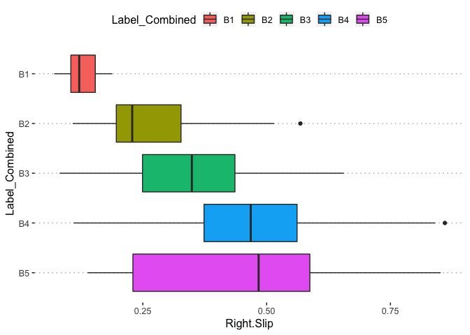
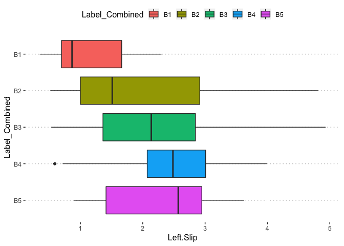
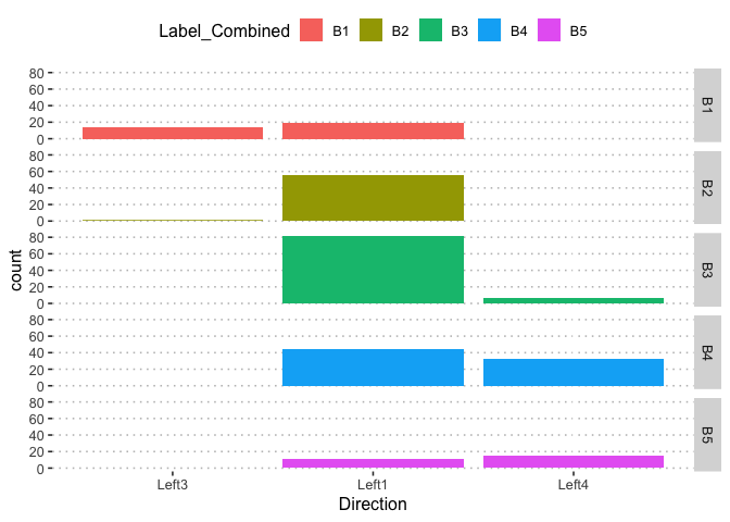
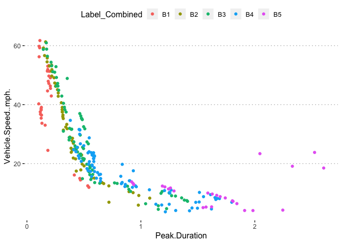
potholedata%>%select(Label_Combined ,Peak.Duration, Vehicle.Speed..mph., Peak.Z.Accel,Peak.Lat.Accel, Peak.Long.Accel,Front.Slip, Right.Slip, Left.Slip, Direction)%>%ggpairs(title = "")+
  theme(legend.position = "top")
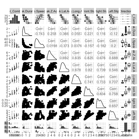
pn<-potholedata%>%select(Label_Combined ,Peak.Duration, Vehicle.Speed..mph., Peak.Z.Accel,Peak.Lat.Accel, Peak.Long.Accel,Front.Slip, Right.Slip, Left.Slip, Direction)%>%ggpairs(title = "",mapping = aes(color = Label_Combined ))+
  theme(legend.position = "top")

pn
We can select the elements in the matrix plot with their indices.
pn[1,1]
pn[1,2]
pn[1,3]
pn[1,4]
pn[1,5]
pn[1,6]
pn[1,7]
pn[1,8]
pn[1,9]
pn[1,10]
pn[3,2]
pn[6,5]

pn[5,3]
pn[6,4]
pn[6,5]
pn[6,3]
The summary statistics for each variable in the data
skimmed <-skim_to_wide(potholedata)
skimmed%>%
  kable() %>%
  kable_styling()
| type | variable | missing | complete | n | min | max | median | n_unique | top_counts | ordered | mean | sd | p0 | p25 | p50 | p75 | p100 | hist |
|---|---|---|---|---|---|---|---|---|---|---|---|---|---|---|---|---|---|---|
| Date | Date | 0 | 280 | 280 | 2018-07-09 | 2018-07-16 | 2018-07-09 | 2 | NA | NA | NA | NA | NA | NA | NA | NA | NA | NA |
| factor | Direction | 0 | 280 | 280 | NA | NA | NA | 3 | Lef: 211, Lef: 54, Lef: 15, NA: 0 | FALSE | NA | NA | NA | NA | NA | NA | NA | NA |
| factor | File | 0 | 280 | 280 | NA | NA | NA | 12 | Cal: 44, Cal: 43, Cal: 37, Cal: 32 | FALSE | NA | NA | NA | NA | NA | NA | NA | NA |
| factor | Label | 0 | 280 | 280 | NA | NA | NA | 9 | P2: 57, P3: 55, P1: 33, P5: 33 | FALSE | NA | NA | NA | NA | NA | NA | NA | NA |
| factor | Label_Combined | 0 | 280 | 280 | NA | NA | NA | 5 | B3: 87, B4: 77, B2: 57, B1: 33 | FALSE | NA | NA | NA | NA | NA | NA | NA | NA |
| factor | MLT1.Feature | 0 | 280 | 280 | NA | NA | NA | 3 | Typ: 166, Typ: 113, Hum: 1, NA: 0 | FALSE | NA | NA | NA | NA | NA | NA | NA | NA |
| factor | MLT2.Feature | 0 | 280 | 280 | NA | NA | NA | 2 | N/A: 279, Cre: 1, NA: 0 | FALSE | NA | NA | NA | NA | NA | NA | NA | NA |
| numeric | Front.Slip | 0 | 280 | 280 | NA | NA | NA | NA | NA | NA | 1.76 | 0.84 | 0.31 | 1.02 | 1.62 | 2.34 | 3.95 | ▅▇▇▅▇▂▂▁ |
| numeric | Left.Slip | 0 | 280 | 280 | NA | NA | NA | NA | NA | NA | 2.12 | 1.08 | 0.35 | 1.24 | 2.08 | 2.85 | 4.93 | ▅▇▆▇▆▃▁▂ |
| numeric | Peak.Duration | 0 | 280 | 280 | NA | NA | NA | NA | NA | NA | 0.68 | 0.51 | 0.1 | 0.32 | 0.5 | 0.92 | 2.6 | ▇▇▂▂▂▁▁▁ |
| numeric | Peak.Lat.Accel | 0 | 280 | 280 | NA | NA | NA | NA | NA | NA | 2.88 | 1.41 | 0.22 | 1.74 | 2.66 | 3.77 | 6.22 | ▂▇▇▇▆▃▃▂ |
| numeric | Peak.Long.Accel | 0 | 280 | 280 | NA | NA | NA | NA | NA | NA | 2.46 | 1.17 | 0.16 | 1.5 | 2.33 | 3.46 | 5.32 | ▂▇▇▇▆▆▃▁ |
| numeric | Peak.Z.Accel | 0 | 280 | 280 | NA | NA | NA | NA | NA | NA | 3.42 | 1.29 | 1.32 | 2.44 | 3.12 | 4.25 | 7.09 | ▅▇▇▅▃▃▂▁ |
| numeric | Right.Slip | 0 | 280 | 280 | NA | NA | NA | NA | NA | NA | 0.34 | 0.18 | 0.071 | 0.19 | 0.33 | 0.46 | 0.86 | ▇▇▆▇▅▃▁▁ |
| numeric | Vehicle.Speed..mph. | 0 | 280 | 280 | NA | NA | NA | NA | NA | NA | 25.36 | 15.58 | 3.64 | 12.45 | 22.55 | 36.22 | 61.73 | ▇▇▇▅▃▂▃▂ |
#skimr::skim(potholedata)

  mlr::summarizeColumns(potholedata)%>%

  kable(escape = F, align = "c") %>%
  kable_styling(c("striped", "condensed"), full_width = F)
| name | type | na | mean | disp | median | mad | min | max | nlevs |
|---|---|---|---|---|---|---|---|---|---|
| Label_Combined | factor | 0 | NA | 0.6892857 | NA | NA | 26.0000000 | 87.0000000 | 5 |
| Label | factor | 0 | NA | 0.7964286 | NA | NA | 13.0000000 | 57.0000000 | 9 |
| Peak.Duration | numeric | 0 | 0.6762429 | 0.5070269 | 0.4985000 | 0.3484110 | 0.1040000 | 2.6050000 | 0 |
| Vehicle.Speed..mph. | numeric | 0 | 25.3645046 | 15.5784650 | 22.5494956 | 16.2697198 | 3.6364981 | 61.7288470 | 0 |
| Peak.Z.Accel | numeric | 0 | 3.4220157 | 1.2917025 | 3.1230914 | 1.2859451 | 1.3170555 | 7.0852490 | 0 |
| Peak.Lat.Accel | numeric | 0 | 2.8756696 | 1.4096700 | 2.6602507 | 1.4832631 | 0.2202256 | 6.2201228 | 0 |
| Peak.Long.Accel | numeric | 0 | 2.4605413 | 1.1737102 | 2.3336269 | 1.3882734 | 0.1579519 | 5.3205001 | 0 |
| Front.Slip | numeric | 0 | 1.7559611 | 0.8388320 | 1.6233722 | 0.9514858 | 0.3131939 | 3.9547484 | 0 |
| Right.Slip | numeric | 0 | 0.3431604 | 0.1764695 | 0.3345577 | 0.2042645 | 0.0711265 | 0.8599148 | 0 |
| Left.Slip | numeric | 0 | 2.1245021 | 1.0781293 | 2.0771931 | 1.1810550 | 0.3469242 | 4.9332445 | 0 |
| Direction | factor | 0 | NA | 0.2464286 | NA | NA | 15.0000000 | 211.0000000 | 3 |
| MLT1.Feature | factor | 0 | NA | 0.4071429 | NA | NA | 1.0000000 | 166.0000000 | 3 |
| MLT2.Feature | factor | 0 | NA | 0.0035714 | NA | NA | 1.0000000 | 279.0000000 | 2 |
| File | factor | 0 | NA | 0.8428571 | NA | NA | 4.0000000 | 44.0000000 | 12 |
| Date | Date | 0 | NA | NA | NA | NA | 4.0000000 | 276.0000000 | 2 |
Model Building
The rsample package can be used to split the data into training and test set.
library(rsample)

pothole_data<-potholedata%>%dplyr::select(-Date,-Label,-File,-Date,-MLT2.Feature)

data_split <- initial_split(pothole_data, strata = "Label_Combined", prop = 0.8)

pothole_train <- training(data_split)
pothole_test  <- testing(data_split)
The recipes package makes prepocessing step in machine learning very convenient. Most preprocessing steps involves one single line of code. The first step is to apply the Yeo-Johnson Power transformation. It is similar to the popular Box-Cox Transformation but includes transformation family of variables that include negative values. We do this transformation to stabilize variance and make the data more normal distribution-like. Next is to center and standardize all numeric variables in the data to a mean of zero and a unit variance. With step-other function we lump factor levels that occur in <= 10% of data as “other”.step-dummy createsone-hot encoding or dummy variables for all nominal predictor factor variables except the response One-hot encoding.
pothole_recipe2 <- recipe(Label_Combined ~ ., data = pothole_train ) %>%
  #Transform numeric skewed predictors
  step_YeoJohnson(all_numeric()) %>%
  # standardize the data
  step_center(all_numeric(), -all_outcomes()) %>%
  #scale the data
  step_scale(all_numeric(), -all_outcomes()) %>%
  #step_kpca a specification of a recipe step that will convert numeric data into one or more principal components using a kernel basis expansion.
  #step_kpca(all_numeric(), num=6)%>%
  #step_log(Label, base = 10)
   # Lump factor levels that occur in <= 10% of data as "other"
  step_other(Direction, MLT1.Feature, threshold = 0.1) %>%
  # Create dummy variables for all nominal predictor factor variables except the response
  step_dummy(all_nominal(), -all_outcomes())%>%
  prep(data = pothole_train,retain = TRUE )

# split data into training and test set
test_tbl2  <- bake(pothole_recipe2, newdata = pothole_test)
train_tbl2 <- bake(pothole_recipe2, newdata = pothole_train)
glimpse(train_tbl2)
## Observations: 226
## Variables: 13
## $ Label_Combined      <fct> B1, B1, B1, B1, B1, B1, B1, B1, B1, B1, B1...
## $ Peak.Duration       <dbl> 0.006525519, -0.207802332, -0.226370118, -...
## $ Vehicle.Speed..mph. <dbl> -0.8249478, -0.5814521, -0.5330513, -0.433...
## $ Peak.Z.Accel        <dbl> -2.1870155, -2.0950290, -2.2040901, -2.189...
## $ Peak.Lat.Accel      <dbl> -1.3096776, -1.0552851, -1.4598802, -1.291...
## $ Peak.Long.Accel     <dbl> -1.85372136, -1.04917684, -1.31762792, -1....
## $ Front.Slip          <dbl> -2.0399125, -1.4628490, -1.3852557, -1.758...
## $ Right.Slip          <dbl> -1.5197233, -1.4290844, -1.2639294, -1.429...
## $ Left.Slip           <dbl> -2.18627766, -1.68674759, -1.52218284, -2....
## $ Direction_Left4     <dbl> 0, 0, 0, 0, 0, 0, 0, 0, 0, 0, 0, 0, 0, 0, ...
## $ Direction_other     <dbl> 1, 0, 0, 1, 1, 1, 0, 1, 1, 1, 1, 0, 1, 1, ...
## $ MLT1.Feature_Type2  <dbl> 0, 0, 0, 0, 0, 0, 0, 0, 0, 0, 0, 0, 0, 0, ...
## $ MLT1.Feature_other  <dbl> 0, 0, 0, 0, 1, 0, 0, 0, 0, 0, 0, 0, 0, 0, ...
Multinomial Logistic Regression
The first model we consider is the multinomial logistic regression. Multinomial logistic regression is used to model nominal outcome variables, in which the log odds of the outcomes are modeled as a linear combination of the predictor variables.
library(ggrepel)
# Fit the multinomial logistic model
model_multlog  <- nnet::multinom(Label_Combined ~., data = train_tbl2)
## # weights:  70 (52 variable)
## initial  value 363.732968
## iter  10 value 186.989385
## iter  20 value 93.855296
## iter  30 value 35.866528
## iter  40 value 32.017762
## iter  50 value 30.831075
## iter  60 value 29.827671
## iter  70 value 29.455249
## iter  80 value 29.228431
## iter  90 value 28.858957
## iter 100 value 28.619521
## final  value 28.619521
## stopped after 100 iterations
#summary(model_multlog )
tidy(model_multlog)%>%
  kable(escape = F, align = "c") %>%
  kable_styling(c("striped", "condensed"), full_width = F)
| y.level | term | estimate | std.error | statistic | p.value |
|---|---|---|---|---|---|
| B2 | (Intercept) | 1.006932e+43 | 123.808721 | 7.997665e-01 | 0.4238461 |
| B2 | Peak.Duration | 6.468647e+18 | 72.453981 | 5.978070e-01 | 0.5499687 |
| B2 | Vehicle.Speed..mph. | 1.104725e+07 | 32.174210 | 5.040587e-01 | 0.6142201 |
| B2 | Peak.Z.Accel | 5.335858e+07 | 164.997240 | 1.078354e-01 | 0.9141263 |
| B2 | Peak.Lat.Accel | 1.119356e+02 | 53.964076 | 8.742710e-02 | 0.9303320 |
| B2 | Peak.Long.Accel | 1.311299e+00 | 20.762958 | 1.305300e-02 | 0.9895855 |
| B2 | Front.Slip | 3.094576e+10 | 134.148466 | 1.800654e-01 | 0.8571012 |
| B2 | Right.Slip | 4.387685e+14 | 107.542443 | 3.135041e-01 | 0.7538977 |
| B2 | Left.Slip | 0.000000e+00 | 147.569783 | -1.478489e-01 | 0.8824620 |
| B2 | Direction_Left4 | 0.000000e+00 | 0.000000 | -1.970507e+09 | 0.0000000 |
| B2 | Direction_other | 5.796511e-01 | 152.479942 | -3.576400e-03 | 0.9971465 |
| B2 | MLT1.Feature_Type2 | 6.878763e+05 | 7.952293 | 1.690250e+00 | 0.0909801 |
| B2 | MLT1.Feature_other | 0.000000e+00 | 0.000000 | -7.021216e+09 | 0.0000000 |
| B3 | (Intercept) | 4.040040e+51 | 123.983569 | 9.584181e-01 | 0.3378520 |
| B3 | Peak.Duration | 1.743407e+18 | 72.251109 | 5.813388e-01 | 0.5610121 |
| B3 | Vehicle.Speed..mph. | 1.023150e-02 | 32.485612 | -1.410558e-01 | 0.8878259 |
| B3 | Peak.Z.Accel | 1.497944e+21 | 165.843708 | 2.940020e-01 | 0.7687564 |
| B3 | Peak.Lat.Accel | 2.493845e+03 | 54.157950 | 1.444217e-01 | 0.8851675 |
| B3 | Peak.Long.Accel | 3.748920e-01 | 20.817928 | -4.712850e-02 | 0.9624108 |
| B3 | Front.Slip | 1.146640e+09 | 134.198452 | 1.554422e-01 | 0.8764727 |
| B3 | Right.Slip | 6.288793e+15 | 107.505841 | 3.383774e-01 | 0.7350788 |
| B3 | Left.Slip | 0.000000e+00 | 147.712431 | -1.929784e-01 | 0.8469758 |
| B3 | Direction_Left4 | 0.000000e+00 | 15.058656 | -3.318957e+00 | 0.0009035 |
| B3 | Direction_other | 0.000000e+00 | 0.000000 | -6.555174e+10 | 0.0000000 |
| B3 | MLT1.Feature_Type2 | 3.297745e+07 | 6.873321 | 2.518627e+00 | 0.0117813 |
| B3 | MLT1.Feature_other | 6.279000e-04 | 0.000000 | -8.836191e+10 | 0.0000000 |
| B4 | (Intercept) | 2.363141e+49 | 124.004944 | 9.167914e-01 | 0.3592520 |
| B4 | Peak.Duration | 4.233409e+16 | 72.255228 | 5.298491e-01 | 0.5962165 |
| B4 | Vehicle.Speed..mph. | 8.000000e-07 | 32.559928 | -4.321252e-01 | 0.6656504 |
| B4 | Peak.Z.Accel | 1.716274e+24 | 165.857570 | 3.364465e-01 | 0.7365342 |
| B4 | Peak.Lat.Accel | 1.288872e+04 | 54.178156 | 1.746849e-01 | 0.8613272 |
| B4 | Peak.Long.Accel | 1.273826e-01 | 20.849234 | -9.883150e-02 | 0.9212721 |
| B4 | Front.Slip | 3.612412e+11 | 134.234403 | 1.982563e-01 | 0.8428446 |
| B4 | Right.Slip | 3.315180e+18 | 107.530926 | 3.965840e-01 | 0.6916743 |
| B4 | Left.Slip | 0.000000e+00 | 147.782400 | -2.586204e-01 | 0.7959281 |
| B4 | Direction_Left4 | 0.000000e+00 | 14.977781 | -3.823875e+00 | 0.0001314 |
| B4 | Direction_other | 3.188615e+11 | 441.523491 | 5.999230e-02 | 0.9521617 |
| B4 | MLT1.Feature_Type2 | 2.136756e+08 | 6.871591 | 2.791198e+00 | 0.0052513 |
| B4 | MLT1.Feature_other | 1.104226e+02 | 0.000000 | 1.040894e+13 | 0.0000000 |
| B5 | (Intercept) | 4.434352e+15 | 147.413209 | 2.444025e-01 | 0.8069191 |
| B5 | Peak.Duration | 2.046723e+27 | 75.591690 | 8.319173e-01 | 0.4054556 |
| B5 | Vehicle.Speed..mph. | 0.000000e+00 | 56.546553 | -7.853381e-01 | 0.4322553 |
| B5 | Peak.Z.Accel | 4.554239e+48 | 176.256593 | 6.356650e-01 | 0.5249948 |
| B5 | Peak.Lat.Accel | 6.726265e+02 | 62.987158 | 1.033733e-01 | 0.9176667 |
| B5 | Peak.Long.Accel | 2.950000e-04 | 26.937573 | -3.017524e-01 | 0.7628408 |
| B5 | Front.Slip | 5.853313e+04 | 145.595906 | 7.539600e-02 | 0.9398996 |
| B5 | Right.Slip | 3.327703e+21 | 108.832751 | 4.553461e-01 | 0.6488603 |
| B5 | Left.Slip | 0.000000e+00 | 162.114774 | -1.253797e-01 | 0.9002230 |
| B5 | Direction_Left4 | 0.000000e+00 | 29.915098 | -2.621409e+00 | 0.0087567 |
| B5 | Direction_other | 5.659578e+34 | 0.000000 | 4.724513e+54 | 0.0000000 |
| B5 | MLT1.Feature_Type2 | 5.638244e-01 | 20.036849 | -2.859790e-02 | 0.9771853 |
| B5 | MLT1.Feature_other | 8.524256e+02 | 0.000000 | 4.544929e+88 | 0.0000000 |
z<-summary(model_multlog)$coefficients/summary(model_multlog)$standard.errors
# 2-tailed z test
 ((1 - pnorm(abs(z), 0, 1)) * 2) %>%
  kable(escape = F, align = "c") %>%
  kable_styling(c("striped", "condensed"), full_width = F)
| (Intercept) | Peak.Duration | Vehicle.Speed..mph. | Peak.Z.Accel | Peak.Lat.Accel | Peak.Long.Accel | Front.Slip | Right.Slip | Left.Slip | Direction_Left4 | Direction_other | MLT1.Feature_Type2 | MLT1.Feature_other | |
|---|---|---|---|---|---|---|---|---|---|---|---|---|---|
| B2 | 0.4238461 | 0.5499687 | 0.6142201 | 0.9141263 | 0.9303320 | 0.9895855 | 0.8571012 | 0.7538977 | 0.8824620 | 0.0000000 | 0.9971465 | 0.0909801 | 0 |
| B3 | 0.3378520 | 0.5610121 | 0.8878259 | 0.7687564 | 0.8851675 | 0.9624108 | 0.8764727 | 0.7350788 | 0.8469758 | 0.0009035 | 0.0000000 | 0.0117813 | 0 |
| B4 | 0.3592520 | 0.5962165 | 0.6656504 | 0.7365342 | 0.8613272 | 0.9212721 | 0.8428446 | 0.6916743 | 0.7959281 | 0.0001314 | 0.9521617 | 0.0052513 | 0 |
| B5 | 0.8069191 | 0.4054556 | 0.4322553 | 0.5249948 | 0.9176667 | 0.7628408 | 0.9398996 | 0.6488603 | 0.9002230 | 0.0087567 | 0.0000000 | 0.9771853 | 0 |
glance(model_multlog) %>%
  kable(escape = F, align = "c") %>%
  kable_styling(c("striped", "condensed"), full_width = F)
| edf | deviance | AIC |
|---|---|---|
| 52 | 57.23904 | 161.239 |
# Make predictions
pred3 = predict(model_multlog , newdata = test_tbl2, type="class")

data1=data.frame(test_tbl2["Label_Combined"],predicted=pred3)

#check accuracy
yardstick::metrics(data1,truth = Label_Combined, estimate = predicted)
## # A tibble: 1 x 1
##   accuracy
##      <dbl>
## 1    0.926
# Make predictions
predicted.classes <- model_multlog  %>% predict(test_tbl2)
head(predicted.classes)
## [1] B1 B1 B2 B1 B1 B3
## Levels: B1 B2 B3 B4 B5
#Equivalently Model accuracy

mean(predicted.classes == test_tbl2$Label_Combined)
## [1] 0.9259259
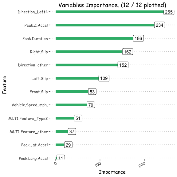
#plot variable importance
feature=factor(rownames(varImp(model_multlog ,scale=T)))
Importance=varImp(model_multlog ,scale=T)$Overall


Varplot(feature,Importance)
ggsave("/POTHOLEDETECTION/variable.png")
#confusion matrix
table(predicted.classes,test_tbl2$Label_Combined)
##
## predicted.classes B1 B2 B3 B4 B5
##                B1  4  0  0  0  0
##                B2  1 14  0  0  0
##                B3  0  1 15  0  0
##                B4  0  0  2 14  0
##                B5  0  0  0  0  3
Multi-class Evaluation Metrics
Macro-Averaging
The overall classification accuracy is defined as the fraction of instances that are correctly classified. In order to assess the performance of a classification,these metrics are calculated from the model predictions. In cases where the class labels are not uniformly distributed or imbalance class labels, using the accuracy metric alone may be misleading as one could predict the dominant class most of the time and still achieve a relatively high overall accuracy but very low precision or recall for other classes.
Specificity or TNR (True Negative Rate): Number of items correctly identified as negative out of total negatives- TN/(TN+FP)
Recall or Sensitivity or TPR (True Positive Rate): Number of items correctly identified as positive out of total true positives- TP/(TP+FN) Precision: Number of items correctly identified as positive out of total items identified as positive- TP/(TP+FP)
**F1 Score:** It is a harmonic mean of precision and recall given by- $F1 = \frac{2*Precision*Recall}{(Precision + Recall)} $
Accuracy: Percentage of total items classified correctly- (TP+TN)/(N+P)
Macro-averaged Metrics
The per-class metrics can be averaged over all the classes resulting in macro-averaged precision, recall and F-1.
model_multlog_pred<-predict(model_multlog , newdata = test_tbl2, type="probs")

#pred <- predict(model_multlog, newdata = test_tbl2, probability = TRUE)

#MLmetrics::MultiLogLoss(y_true = test_tbl2$Label_Combined, y_pred = attr(model_multlog_pred, "probabilities"))
Overall Classification Accuracy
l=caret::confusionMatrix(predicted.classes,test_tbl2$Label_Combined)

overall_classification_accuracy<-sum(diag(l$table))/sum(l$table)

l$overall%>%data.frame()%>%
  rename(`Macro Measure`=".")%>%
  kable(escape = F, align = "c") %>%
  kable_styling(c("striped", "condensed"), full_width = F)
| Macro Measure | |
|---|---|
| Accuracy | 0.9259259 |
| Kappa | 0.9002770 |
| AccuracyLower | 0.8210666 |
| AccuracyUpper | 0.9794490 |
| AccuracyNull | 0.3148148 |
| AccuracyPValue | 0.0000000 |
| McnemarPValue | NaN |
Per-class Precision, Recall, and F-1
l$byClass%>%
  kable(escape = F, align = "c") %>%
  kable_styling(c("striped", "condensed"), full_width = F)
| Sensitivity | Specificity | Pos Pred Value | Neg Pred Value | Precision | Recall | F1 | Prevalence | Detection Rate | Detection Prevalence | Balanced Accuracy | |
|---|---|---|---|---|---|---|---|---|---|---|---|
| Class: B1 | 0.8000000 | 1.000000 | 1.0000000 | 0.9800000 | 1.0000000 | 0.8000000 | 0.8888889 | 0.0925926 | 0.0740741 | 0.0740741 | 0.9000000 |
| Class: B2 | 0.9333333 | 0.974359 | 0.9333333 | 0.9743590 | 0.9333333 | 0.9333333 | 0.9333333 | 0.2777778 | 0.2592593 | 0.2777778 | 0.9538462 |
| Class: B3 | 0.8823529 | 0.972973 | 0.9375000 | 0.9473684 | 0.9375000 | 0.8823529 | 0.9090909 | 0.3148148 | 0.2777778 | 0.2962963 | 0.9276630 |
| Class: B4 | 1.0000000 | 0.950000 | 0.8750000 | 1.0000000 | 0.8750000 | 1.0000000 | 0.9333333 | 0.2592593 | 0.2592593 | 0.2962963 | 0.9750000 |
| Class: B5 | 1.0000000 | 1.000000 | 1.0000000 | 1.0000000 | 1.0000000 | 1.0000000 | 1.0000000 | 0.0555556 | 0.0555556 | 0.0555556 | 1.0000000 |
Macro-averaged Metrics
macro_meaure=l$byClass%>%apply(.,2,mean)%>%
  data.frame()%>%
  rename(`Macro Measure`=".")

macro_meaure%>%
  kable(escape = F, align = "c") %>%
  kable_styling(c("striped", "condensed"), full_width = F)
| Macro Measure | |
|---|---|
| Sensitivity | 0.9231373 |
| Specificity | 0.9794664 |
| Pos Pred Value | 0.9491667 |
| Neg Pred Value | 0.9803455 |
| Precision | 0.9491667 |
| Recall | 0.9231373 |
| F1 | 0.9329293 |
| Prevalence | 0.2000000 |
| Detection Rate | 0.1851852 |
| Detection Prevalence | 0.2000000 |
| Balanced Accuracy | 0.9513018 |
The confusion matrix is given as:
l$table%>%
  kable(escape = F, align = "c") %>%
  kable_styling(c("striped", "condensed"), full_width = F)
| B1 | B2 | B3 | B4 | B5 | |
|---|---|---|---|---|---|
| B1 | 4 | 0 | 0 | 0 | 0 |
| B2 | 1 | 14 | 0 | 0 | 0 |
| B3 | 0 | 1 | 15 | 0 | 0 |
| B4 | 0 | 0 | 2 | 14 | 0 |
| B5 | 0 | 0 | 0 | 0 | 3 |
The function below can be used to find the multi-class logloss. Logloss is among the numerous evaluation metric for multi-class classfication models.
pred_probs1<-predict(model_multlog , newdata = test_tbl2, type="probs")

#truth: integer vector with truth labels, values range from 0 to n - 1 classes
 # prob_matrix: predicted probs: column 1 => label 0, column 2 => label 1 and so on
  Multiclasslogloss = function(truth, pred_prob_matrix, eps = 1e-15){

     if(is.double(truth)=="FALSE"){

     truth=as.numeric(truth)-1

    }


    if(max(truth) >= ncol(pred_prob_matrix) || min(truth) < 0){
      stop(cat('True labels should range from 0 to', ncol(pred_prob_matrix) - 1, '\n'))
    }


   pred_prob_matrix[pred_prob_matrix > 1 - eps] = 1 - eps
   pred_prob_matrix[pred_prob_matrix< eps] = eps
   pred_prob_matrix = t(apply(pred_prob_matrix, 1, function(r)r/sum(r)))
   truth_matrix = matrix(0, nrow = nrow(pred_prob_matrix), ncol = ncol(pred_prob_matrix))
   truth_matrix[matrix(c(1:nrow(pred_prob_matrix), truth + 1), ncol = 2)] = 1
   -sum(truth_matrix * log(pred_prob_matrix))/nrow(pred_prob_matrix)
  }


Multiclasslogloss(test_tbl2$Label_Combined, pred_probs1)
## [1] 0.3282304
Micro-averaged Metrics
The micro-averaged precision, recall, and F-1 can also be computed from the matrix above. Compared to unweighted macro-averaging, micro-averaging favors classes with a larger number of instances. Because the sum of the one-vs-all matrices is a symmetric matrix, the micro-averaged precision, recall, and F-1 wil be the same.
 n = sum(l$table) # number of instances
 nc = nrow(l$table) # number of classes
 diag = diag(l$table) # number of correctly classified instances per class
 rowsums = apply(l$table, 1, sum) # number of instances per class
 colsums = apply(l$table, 2, sum) # number of predictions per class
 p = rowsums / n # distribution of instances over the actual classes
 q = colsums / n # distribution of instances over the predicted classes

precision = diag / colsums
recall = diag / rowsums
f1 = 2 * precision * recall / (precision + recall)
data.frame(precision, recall, f1)
##    precision    recall        f1
## B1 0.8000000 1.0000000 0.8888889
## B2 0.9333333 0.9333333 0.9333333
## B3 0.8823529 0.9375000 0.9090909
## B4 1.0000000 0.8750000 0.9333333
## B5 1.0000000 1.0000000 1.0000000
One-vs-all
For micro-averaging metrics , we can examine the performance of the classifier one class at a time. This results in 5 binary classification task such that the class considered is the positive class and all others constitute the negative class.
pacman::p_load(furrr)


### faster version using furrr package
oneVsAll =furrr::future_map(1 : nc,
                      function(i){
                        m = c(l$table[i,i],
                              rowsums[i] - l$table[i,i],
                              colsums[i] - l$table[i,i],
                              n-rowsums[i] - colsums[i] + l$table[i,i]);
                        return(matrix(m, nrow = 2, byrow = T))})


#sum matrices element wise
#s=rowSums(c, dims = 2)


#equivalenlty
#apply(c, c(1,2), sum)


## A general-purpose adder:
#this function adds the elements of the matrix
#in the list elementwise
add <- function(x) Reduce("+", x)
sum_all<-add(oneVsAll)
Average Accuracy
Similar to the overall accuracy, the average accuracy is defined as the fraction of correctly classified instances in the sum of one-vs-all matrices matrix.
Average_Accuracy <- sum(diag(sum_all)) / sum(sum_all)

Average_Accuracy
## [1] 0.9703704
Micro-averaged Metrics
The micro-averaged precision, recall, and F-1 can also be computed from the matrix above. Compared to unweighted macro-averaging, micro-averaging favors classes with a larger number of instances. Because the sum of the one-vs-all matrices is a symmetric matrix, the micro-averaged precision, recall, and F-1 wil be the same.
Micro_Accuracy<-(diag(sum_all) / apply(sum_all,1, sum))[1];
Micro_Accuracy
## [1] 0.9259259
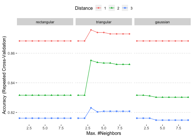
Weighted k-Nearest Neighbor Classifier
The Weighted k-Nearest Neighbor method expands k-nearest neighbor in several directions.It is used for both classification,ordinal classfication and regression. It uses kernel functions to weight the neighbors according to their distances.
fitControl <- trainControl(method="repeatedcv",
 #For repeated k-fold cross-validation only: the number of complete sets of folds to compute
                     repeats = 10,
                     savePredictions = "final",
                     classProbs=TRUE,
          #Either the number of folds or number of resampling iterations
                     number = 10,
                     summaryFunction=multiClassSummary,
                     allowParallel=TRUE)
knn_grid <- expand.grid(
  kmax = 1:9,
  distance = 1:3,
  kernel = c("rectangular", "triangular", "gaussian")
  )


knnFit <- caret::train(Label_Combined ~ .,
                       data = train_tbl2,
                       method = "kknn",
                       trControl = fitControl,
                       tuneGrid = knn_grid,
                       summaryFunction=multiClassSummary,
                        ## Specify which metric to optimize
                        metric = "Accuracy")

#Output of kNN fit
knnFit
## k-Nearest Neighbors
##
## 226 samples
##  12 predictor
##   5 classes: 'B1', 'B2', 'B3', 'B4', 'B5'
##
## No pre-processing
## Resampling: Cross-Validated (10 fold, repeated 10 times)
## Summary of sample sizes: 204, 205, 203, 204, 204, 202, ...
## Resampling results across tuning parameters:
##
##   kmax  distance  kernel       logLoss   AUC        prAUC       Accuracy
##   1     1         rectangular  4.548771  0.9162104  0.06699458  0.8682996
##   1     1         triangular   4.548771  0.9162104  0.06699458  0.8682996
##   1     1         gaussian     4.548771  0.9162104  0.06699458  0.8682996
##   1     2         rectangular  5.815951  0.8920005  0.08356107  0.8316110
##   1     2         triangular   5.815951  0.8920005  0.08356107  0.8316110
##   1     2         gaussian     5.815951  0.8920005  0.08356107  0.8316110
##   1     3         rectangular  6.352123  0.8835768  0.08867452  0.8160872
##   1     3         triangular   6.352123  0.8835768  0.08867452  0.8160872
##   1     3         gaussian     6.352123  0.8835768  0.08867452  0.8160872
##   2     1         rectangular  4.548771  0.9162104  0.06699458  0.8682996


##   Kappa      Mean_F1    Mean_Sensitivity  Mean_Specificity
##   0.8277033  0.8707264  0.8669524         0.9654684
##   0.8277033  0.8707264  0.8669524         0.9654684
##   0.8277033  0.8707264  0.8669524         0.9654684
##   0.7792944  0.8375603  0.8288476         0.9551534
##   0.7792944  0.8375603  0.8288476         0.9551534
##   0.7792944  0.8375603  0.8288476         0.9551534
##   0.7592663  0.8232414  0.8160048         0.9511489
##   0.7592663  0.8232414  0.8160048         0.9511489
##   0.7592663  0.8232414  0.8160048         0.9511489
##   0.8277033  0.8707264  0.8669524         0.9654684


##   Mean_Pos_Pred_Value  Mean_Neg_Pred_Value  Mean_Precision  Mean_Recall
##   0.8911250            0.9669165            0.8911250       0.8669524
##   0.8911250            0.9669165            0.8911250       0.8669524
##   0.8911250            0.9669165            0.8911250       0.8669524
##   0.8664536            0.9575990            0.8664536       0.8288476
##   0.8664536            0.9575990            0.8664536       0.8288476
##   0.8664536            0.9575990            0.8664536       0.8288476
##   0.8534597            0.9538081            0.8534597       0.8160048
##   0.8534597            0.9538081            0.8534597       0.8160048
##   0.8534597            0.9538081            0.8534597       0.8160048
##   0.8911250            0.9669165            0.8911250       0.8669524


##   Mean_Detection_Rate  Mean_Balanced_Accuracy
##   0.1736599            0.9162104
##   0.1736599            0.9162104
##   0.1736599            0.9162104
##   0.1663222            0.8920005
##   0.1663222            0.8920005
##   0.1663222            0.8920005
##   0.1632174            0.8835768
##   0.1632174            0.8835768
##   0.1632174            0.8835768
##   0.1736599            0.9162104


## Accuracy was used to select the optimal model using the largest value.
## The final values used for the model were kmax = 3, distance = 1 and
##  kernel = triangular.
getTrainPerf(knnFit)
##   TrainlogLoss  TrainAUC TrainprAUC TrainAccuracy TrainKappa TrainMean_F1
## 1     2.647393 0.9457703  0.2740201     0.8757911  0.8374018    0.8769454
##   TrainMean_Sensitivity TrainMean_Specificity TrainMean_Pos_Pred_Value
## 1             0.8727143             0.9674464                    0.897
##   TrainMean_Neg_Pred_Value TrainMean_Precision TrainMean_Recall
## 1                0.9689589               0.897        0.8727143
##   TrainMean_Detection_Rate TrainMean_Balanced_Accuracy method
## 1                0.1751582                   0.9200803   kknn
ggplot(knnFit)
saveRDS(knnFit , "/POTHOLEDETECTION/knnFit.rds")
knnFit <- readRDS("/POTHOLEDETECTION/knnFit.rds")
kknnpred1 = predict(knnFit, newdata = test_tbl2, type="prob")
kknnpred = predict(knnFit, newdata = test_tbl2, type="raw")


library(yardstick)

# Compute the summary statistics
d2=data.frame(test_tbl2["Label_Combined"],predicted=kknnpred)
yardstick::metrics(d2,truth = Label_Combined, estimate = predicted)
## # A tibble: 1 x 1
##   accuracy
##      <dbl>
## 1    0.833
yardstick::conf_mat(d2,truth = Label_Combined, estimate = predicted)
##           Truth
## Prediction B1 B2 B3 B4 B5
##         B1  5  2  0  0  0
##         B2  0 10  1  0  0
##         B3  0  3 15  1  0
##         B4  0  0  1 12  0
##         B5  0  0  0  1  3
l=caret::confusionMatrix(kknnpred,test_tbl2$Label_Combined)


l$overall%>%data.frame()%>%
  rename(`Macro Measure`=".")%>%
  kable(escape = F, align = "c") %>%
  kable_styling(c("striped", "condensed"), full_width = F)
| Macro Measure | |
|---|---|
| Accuracy | 0.8333333 |
| Kappa | 0.7789905 |
| AccuracyLower | 0.7070588 |
| AccuracyUpper | 0.9208456 |
| AccuracyNull | 0.3148148 |
| AccuracyPValue | 0.0000000 |
| McnemarPValue | NaN |
l$byClass%>%
  kable(escape = F, align = "c") %>%
  kable_styling(c("striped", "condensed"), full_width = F)
| Sensitivity | Specificity | Pos Pred Value | Neg Pred Value | Precision | Recall | F1 | Prevalence | Detection Rate | Detection Prevalence | Balanced Accuracy | |
|---|---|---|---|---|---|---|---|---|---|---|---|
| Class: B1 | 1.0000000 | 0.9591837 | 0.7142857 | 1.0000000 | 0.7142857 | 1.0000000 | 0.8333333 | 0.0925926 | 0.0925926 | 0.1296296 | 0.9795918 |
| Class: B2 | 0.6666667 | 0.9743590 | 0.9090909 | 0.8837209 | 0.9090909 | 0.6666667 | 0.7692308 | 0.2777778 | 0.1851852 | 0.2037037 | 0.8205128 |
| Class: B3 | 0.8823529 | 0.8918919 | 0.7894737 | 0.9428571 | 0.7894737 | 0.8823529 | 0.8333333 | 0.3148148 | 0.2777778 | 0.3518519 | 0.8871224 |
| Class: B4 | 0.8571429 | 0.9750000 | 0.9230769 | 0.9512195 | 0.9230769 | 0.8571429 | 0.8888889 | 0.2592593 | 0.2222222 | 0.2407407 | 0.9160714 |
| Class: B5 | 1.0000000 | 0.9803922 | 0.7500000 | 1.0000000 | 0.7500000 | 1.0000000 | 0.8571429 | 0.0555556 | 0.0555556 | 0.0740741 | 0.9901961 |
macro_meaure=l$byClass%>%apply(.,2,mean)%>%
  data.frame()%>%
  rename(`Macro Measure`=".")

macro_meaure%>%
  kable(escape = F, align = "c") %>%
  kable_styling(c("striped", "condensed"), full_width = F)
| Macro Measure | |
|---|---|
| Sensitivity | 0.8812325 |
| Specificity | 0.9561653 |
| Pos Pred Value | 0.8171854 |
| Neg Pred Value | 0.9555595 |
| Precision | 0.8171854 |
| Recall | 0.8812325 |
| F1 | 0.8363858 |
| Prevalence | 0.2000000 |
| Detection Rate | 0.1666667 |
| Detection Prevalence | 0.2000000 |
| Balanced Accuracy | 0.9186989 |
Multiclasslogloss(test_tbl2$Label_Combined, kknnpred1)
## [1] 2.122451
Multinomial Logistic Regression with H20
The h2o.glm function can be used to fit multinomial logistic regression and a host of other generalized linear regression models including poisson, ordinal ,ridge and LASSO.
library(h2o)
h2o.init()
##  Connection successful!
##
## R is connected to the H2O cluster:
##     H2O cluster uptime:         1 days 13 hours
##     H2O cluster timezone:       America/Detroit
##     H2O data parsing timezone:  UTC
##     H2O cluster version:        3.20.0.2
##     H2O cluster version age:    2 months and 5 days
##     H2O cluster name:           H2O_started_from_R_nanaakwasiabayieboateng_par282
##     H2O cluster total nodes:    1
##     H2O cluster total memory:   1.54 GB
##     H2O cluster total cores:    8
##     H2O cluster allowed cores:  8
##     H2O cluster healthy:        TRUE
##     H2O Connection ip:          localhost
##     H2O Connection port:        54321
##     H2O Connection proxy:       NA
##     H2O Internal Security:      FALSE
##     H2O API Extensions:         XGBoost, Algos, AutoML, Core V3, Core V4
##     R Version:                  R version 3.5.0 (2018-04-23)
pf=as.h2o(train_tbl2)
##
  |
  |                                                                 |   0%
  |
  |=================================================================| 100%
pftest=as.h2o(test_tbl2)
##
  |
  |                                                                 |   0%
  |
  |=================================================================| 100%
# Run GLM
myX = setdiff(colnames(train_tbl2), "Label_Combined")

h2o_mult<-h2o.glm(y = "Label_Combined", x = myX, training_frame = pf, family = "multinomial",
nfolds = 0, alpha = 0, lambda_search = FALSE)
##
  |
  |                                                                 |   0%
  |
  |=================================================================| 100%
h2o.performance(h2o_mult)
## H2OMultinomialMetrics: glm
## ** Reported on training data. **
##
## Training Set Metrics:
## =====================
##
## Extract training frame with `h2o.getFrame("train_tbl2")`
## MSE: (Extract with `h2o.mse`) 0.05720497
## RMSE: (Extract with `h2o.rmse`) 0.2391756
## Logloss: (Extract with `h2o.logloss`) 0.2008426
## Mean Per-Class Error: 0.06190476
## Null Deviance: (Extract with `h2o.nulldeviance`) 688.4571
## Residual Deviance: (Extract with `h2o.residual_deviance`) 90.78083
## R^2: (Extract with `h2o.r2`) 0.9580881
## AIC: (Extract with `h2o.aic`) NaN
## Confusion Matrix: Extract with `h2o.confusionMatrix(<model>,train = TRUE)`)
## =========================================================================
## Confusion Matrix: Row labels: Actual class; Column labels: Predicted class
##        B1 B2 B3 B4 B5  Error       Rate
## B1     28  0  0  0  0 0.0000 =   0 / 28
## B2      1 39  2  0  0 0.0714 =   3 / 42
## B3      0  3 60  7  0 0.1429 =  10 / 70
## B4      0  0  6 57  0 0.0952 =   6 / 63
## B5      0  0  0  0 23 0.0000 =   0 / 23
## Totals 29 42 68 64 23 0.0841 = 19 / 226
##
## Hit Ratio Table: Extract with `h2o.hit_ratio_table(<model>,train = TRUE)`
## =======================================================================
## Top-5 Hit Ratios:
##   k hit_ratio
## 1 1  0.915929
## 2 2  1.000000
## 3 3  1.000000
## 4 4  1.000000
## 5 5  1.000000
pftest=as.h2o(test_tbl2)
##
  |
  |                                                                 |   0%
  |
  |=================================================================| 100%
predh20mult=h2o.predict(h2o_mult,pftest)
##
  |
  |                                                                 |   0%
  |
  |=================================================================| 100%
predict_model.H2OMultinomialModel <- function(x, newdata, type, ...) {


# Function performs prediction and returns dataframe with Response

# x is h2o model
# newdata is data frame
# type is only setup for data frame

    pred <- h2o.predict(x, as.h2o(newdata))

    # return classification probabilities only
    return(as.data.frame(pred[,-1]))

}

h2ologisticpred=predict_model.H2OMultinomialModel(h2o_mult,pftest)
##
  |
  |                                                                 |   0%
  |
  |=================================================================| 100%
h2o_multdata<-data.frame(h2o.varimp(h2o_mult))


Varplot(feature=h2o_multdata$names,Importance=h2o_multdata$coefficients)
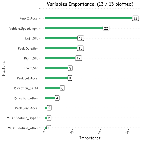
ggsave("/POTHOLEDETECTION/h2o_multcombined.png")
Metric Evaluation
# predicted probabilities for each class
head(h2ologisticpred)
##           B1           B2           B3           B4           B5
## 1 0.97217723 2.776202e-02 6.074508e-05 4.476462e-09 5.842084e-21
## 2 0.99993751 6.248919e-05 1.404794e-13 3.751218e-19 2.523806e-33
## 3 0.15851847 8.404513e-01 1.030224e-03 2.189931e-09 5.605275e-23
## 4 0.98302422 1.697135e-02 4.427456e-06 4.436548e-14 7.376240e-28
## 5 0.98546664 1.453336e-02 1.128159e-09 2.050341e-15 4.547862e-28
## 6 0.02611215 4.125397e-01 5.542656e-01 7.082515e-03 2.472140e-10
#select the indices of the column on rows  of the class with the highest predicted probability as the class label prediction


x=apply(h2ologisticpred, 1, which.max)

prob=apply(h2ologisticpred,1,max)


## Equivalent  way to convert numeric values to factor variables with dplyr
# recode works better, it preserves levels in the factors
y=recode_factor(x, `1` = "B1", `2` = "B2", `3` = "B3",`4` = "B4", `5` = "B5")


probdataframe<-data.frame(x=x,prob=prob,predclass=y)

#accuracy

mean(test_tbl2$Label_Combined==probdataframe$predclass)
## [1] 0.8703704
l=caret::confusionMatrix(probdataframe$predclass,test_tbl2$Label_Combined)


l$overall%>%data.frame()%>%
  rename(`Macro Measure`=".")%>%
  kable(escape = F, align = "c") %>%
  kable_styling(c("striped", "condensed"), full_width = F)
| Macro Measure | |
|---|---|
| Accuracy | 0.8703704 |
| Kappa | 0.8269231 |
| AccuracyLower | 0.7509878 |
| AccuracyUpper | 0.9462570 |
| AccuracyNull | 0.3148148 |
| AccuracyPValue | 0.0000000 |
| McnemarPValue | NaN |
l$byClass%>%
  kable(escape = F, align = "c") %>%
  kable_styling(c("striped", "condensed"), full_width = F)
| Sensitivity | Specificity | Pos Pred Value | Neg Pred Value | Precision | Recall | F1 | Prevalence | Detection Rate | Detection Prevalence | Balanced Accuracy | |
|---|---|---|---|---|---|---|---|---|---|---|---|
| Class: B1 | 0.8000000 | 0.9591837 | 0.6666667 | 0.9791667 | 0.6666667 | 0.8000000 | 0.7272727 | 0.0925926 | 0.0740741 | 0.1111111 | 0.8795918 |
| Class: B2 | 0.7333333 | 0.9743590 | 0.9166667 | 0.9047619 | 0.9166667 | 0.7333333 | 0.8148148 | 0.2777778 | 0.2037037 | 0.2222222 | 0.8538462 |
| Class: B3 | 0.8823529 | 0.9459459 | 0.8823529 | 0.9459459 | 0.8823529 | 0.8823529 | 0.8823529 | 0.3148148 | 0.2777778 | 0.3148148 | 0.9141494 |
| Class: B4 | 1.0000000 | 0.9500000 | 0.8750000 | 1.0000000 | 0.8750000 | 1.0000000 | 0.9333333 | 0.2592593 | 0.2592593 | 0.2962963 | 0.9750000 |
| Class: B5 | 1.0000000 | 1.0000000 | 1.0000000 | 1.0000000 | 1.0000000 | 1.0000000 | 1.0000000 | 0.0555556 | 0.0555556 | 0.0555556 | 1.0000000 |
macro_meaure=l$byClass%>%apply(.,2,mean)%>%
  data.frame()%>%
  rename(`Macro Measure`=".")

macro_meaure%>%
  kable(escape = F, align = "c") %>%
  kable_styling(c("striped", "condensed"), full_width = F)
| Macro Measure | |
|---|---|
| Sensitivity | 0.8831373 |
| Specificity | 0.9658977 |
| Pos Pred Value | 0.8681373 |
| Neg Pred Value | 0.9659749 |
| Precision | 0.8681373 |
| Recall | 0.8831373 |
| F1 | 0.8715548 |
| Prevalence | 0.2000000 |
| Detection Rate | 0.1740741 |
| Detection Prevalence | 0.2000000 |
| Balanced Accuracy | 0.9245175 |
Multiclasslogloss(test_tbl2$Label_Combined, as.matrix(predh20mult[,-1]))
## [1] 0.2677523
Extreme Gradient Boosting Machines
Gradient boosting is a popular machine learning lagorithm for regression and classification problems. It produces a prediction model in the form of an ensemble of weak prediction models using a baselearner such as decision tree. It builds the model in a stage-wise fashion similar to other boosting methods, and then generalizes them by allowing optimization of an arbitrary differentiable loss function. The XGBoost implementation of Gradient Boosting uses a more regularized model formalization to control over-fitting. This gives it a better performance and reduces overfitting.
xgbmGrid <-  expand.grid(max_depth = c(1, 5, 8,10),
                         nrounds=300,
                        colsample_bytree = c(0.3,0.4,0.5,0.6,0.8,1),
                        eta = seq.int(from=0.01, to=0.3, length.out=5),
                        min_child_weight = 1:3,
                        subsample=1,

                        #rate_drop=0.1,
                        #skip_drop=0.1
                        gamma=0.001
                        )

xgbm <-caret::train(Label_Combined ~ ., data = train_tbl2,
                 method = "xgbTree",
                 trControl = fitControl,
                 verbose = FALSE,
                 ## Now specify the exact models
                 ## to evaluate:
                  #summaryFunction=multiClassSummary,
                 tuneGrid = xgbmGrid)


saveRDS(xgbm , "/POTHOLEDETECTION/xgbm.rds")
xgbm <- readRDS("/POTHOLEDETECTION/xgbm.rds")


getTrainPerf(xgbm)
##   TrainlogLoss  TrainAUC TrainprAUC TrainAccuracy TrainKappa TrainMean_F1
## 1    0.3601013 0.9821397  0.6814514      0.868236  0.8277019    0.8726167
##   TrainMean_Sensitivity TrainMean_Specificity TrainMean_Pos_Pred_Value
## 1             0.8734095             0.9649483                0.8925939
##   TrainMean_Neg_Pred_Value TrainMean_Precision TrainMean_Recall
## 1                0.9663713           0.8925939        0.8734095
##   TrainMean_Detection_Rate TrainMean_Balanced_Accuracy  method
## 1                0.1736472                   0.9191789 xgbTree
ggplot(xgbm)
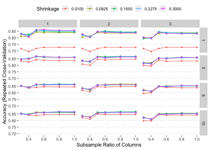
xgbm$bestTune
##     nrounds max_depth    eta gamma colsample_bytree min_child_weight
## 122     300         8 0.0825 0.001              0.8                2
##     subsample
## 122         1
xgbm_pred = predict(xgbm, newdata = test_tbl2, type="raw")
xgbm_pred1 = predict(xgbm, newdata = test_tbl2, type="prob")


xgbmd=data.frame(test_tbl2["Label_Combined"],predicted=xgbm_pred)
yardstick::metrics(xgbmd,truth = Label_Combined, estimate = predicted)
## # A tibble: 1 x 1
##   accuracy
##      <dbl>
## 1    0.907
l=caret::confusionMatrix(xgbm_pred,test_tbl2$Label_Combined)


l$overall%>%data.frame()%>%
  rename(`Macro Measure`=".")%>%
  kable(escape = F, align = "c") %>%
  kable_styling(c("striped", "condensed"), full_width = F)
| Macro Measure | |
|---|---|
| Accuracy | 0.9074074 |
| Kappa | 0.8756333 |
| AccuracyLower | 0.7969985 |
| AccuracyUpper | 0.9692472 |
| AccuracyNull | 0.3148148 |
| AccuracyPValue | 0.0000000 |
| McnemarPValue | NaN |
l$byClass%>%
  kable(escape = F, align = "c") %>%
  kable_styling(c("striped", "condensed"), full_width = F)
| Sensitivity | Specificity | Pos Pred Value | Neg Pred Value | Precision | Recall | F1 | Prevalence | Detection Rate | Detection Prevalence | Balanced Accuracy | |
|---|---|---|---|---|---|---|---|---|---|---|---|
| Class: B1 | 0.8000000 | 0.9795918 | 0.8000000 | 0.9795918 | 0.8000000 | 0.8000000 | 0.8000000 | 0.0925926 | 0.0740741 | 0.0925926 | 0.8897959 |
| Class: B2 | 0.8000000 | 0.9743590 | 0.9230769 | 0.9268293 | 0.9230769 | 0.8000000 | 0.8571429 | 0.2777778 | 0.2222222 | 0.2407407 | 0.8871795 |
| Class: B3 | 0.9411765 | 0.9459459 | 0.8888889 | 0.9722222 | 0.8888889 | 0.9411765 | 0.9142857 | 0.3148148 | 0.2962963 | 0.3333333 | 0.9435612 |
| Class: B4 | 1.0000000 | 0.9750000 | 0.9333333 | 1.0000000 | 0.9333333 | 1.0000000 | 0.9655172 | 0.2592593 | 0.2592593 | 0.2777778 | 0.9875000 |
| Class: B5 | 1.0000000 | 1.0000000 | 1.0000000 | 1.0000000 | 1.0000000 | 1.0000000 | 1.0000000 | 0.0555556 | 0.0555556 | 0.0555556 | 1.0000000 |
macro_meaure=l$byClass%>%apply(.,2,mean)%>%
  data.frame()%>%
  rename(`Macro Measure`=".")

macro_meaure%>%
  kable(escape = F, align = "c") %>%
  kable_styling(c("striped", "condensed"), full_width = F)
| Macro Measure | |
|---|---|
| Sensitivity | 0.9082353 |
| Specificity | 0.9749794 |
| Pos Pred Value | 0.9090598 |
| Neg Pred Value | 0.9757287 |
| Precision | 0.9090598 |
| Recall | 0.9082353 |
| F1 | 0.9073892 |
| Prevalence | 0.2000000 |
| Detection Rate | 0.1814815 |
| Detection Prevalence | 0.2000000 |
| Balanced Accuracy | 0.9416073 |
Multiclasslogloss(test_tbl2$Label_Combined, xgbm_pred1)
## [1] 0.263521
Conclusion
The multinomial logistic regression has superior performance over the machine learning algorithms evaluated in this project. It’s evaluation metrics including accuracy, F-1 score, sensitivity, specificity and precision is higher than for the other models considered.