#<body style="background: #fff;">
Introduction
In this post, I would like to go through some common methods of data exploration. Data exploration is one of the introductory analysis that is performed before any model building task. Data exploration can uncover some hidden patterns and lead to insights into the some phenomenom behind the data.It can inform the selection of appropriate statistical techniques,tools and models. Exploratory techniques are also important for eliminating or sharpening potential hypotheses about the causes of the observed phenomena in the data. We can also detect outliers and anomalies in the data through exploration. Exploratory analysis emphasizes graphical visualizations of the data.
Load Required Packages
The pacman package provides a convenient way to load packages. It installs the package before loading if it not already installed.One of my favorite themes that I use with ggplot is the theme_pubclean. Here I set all themes with ggplot by it.
#install.packages("ggpubr")


#install_github("kassambara/easyGgplot2")
#p_install_gh("kassambara/easyGgplot2")

pacman::p_load(tidyverse,janitor,DataExplorer,skimr,ggpubr,viridis,kableExtra,Amelia,easyGgplot2,VIM)


theme_set(theme_pubclean())
The data for this analysis Orange Juice data, is contained in the ISLR package.The ISLR package created to store the data for the popular introductory statistical learning text, Introduction to Statistical Learning with Applications in R (Gareth James, Daniela Witten, Trevor Hastie and Rob Tibshirani).The data contains 1070 purchases where the customer either purchased Citrus Hill or Minute Maid Orange Juice. A number of characteristics of the customer and product are recorded.The categorical response variable is Purchase with levels CH and MM indicating whether the customer purchased Citrus Hill or Minute Maid Orange Juice. The goal of this data is to predict which of the two brands of orange juice did customers want to buy based on some seventeen features which describes the product and nature of the customers. The dataset can be downloaded here. It contains 1070 observations and seveenteen features plus the response variable purchase.
Description of Variables:
- WeekofPurchase: Week of purchase
- StoreID: Store ID
- PriceCH: Price charged for CH
- PriceMM: Price charged for MM
- DiscCH: Discount offered for CH
- DiscMM: Discount offered for MM
- SpecialCH: Indicator of special on CH
- SpecialMM: Indicator of special on MM
- LoyalCH: Customer brand loyalty for CH
- SalePriceMM: Sale price for MM
- SalePriceCH: Sale price for CH
- PriceDiff: Sale price of MM less sale price of CH
- Store7: A factor with levels No and Yes indicating whether the sale is at Store 7
- PctDiscMM: Percentage discount for MM
- PctDiscCH: Percentage discount for CH
- ListPriceDiff: List price of MM less list price of CH
- STORE: store id.
# Import dataset
orangejuice<-read_csv('https://raw.githubusercontent.com/NanaAkwasiAbayieBoateng/ExploratoryDataAnalysis/master/orangejuice.csv')

write_csv(orangejuice,"orangejuice.csv")

orangejuice%>%head()%>%
  kable(escape = F, align = "c") %>%
  kable_styling(c("striped", "condensed"), full_width = F)
| Purchase | WeekofPurchase | StoreID | PriceCH | PriceMM | DiscCH | DiscMM | SpecialCH | SpecialMM | LoyalCH | SalePriceMM | SalePriceCH | PriceDiff | Store7 | PctDiscMM | PctDiscCH | ListPriceDiff | STORE |
|---|---|---|---|---|---|---|---|---|---|---|---|---|---|---|---|---|---|
| CH | 237 | 1 | 1.75 | 1.99 | 0.00 | 0.0 | 0 | 0 | 0.500000 | 1.99 | 1.75 | 0.24 | No | 0.000000 | 0.000000 | 0.24 | 1 |
| CH | 239 | 1 | 1.75 | 1.99 | 0.00 | 0.3 | 0 | 1 | 0.600000 | 1.69 | 1.75 | -0.06 | No | 0.150754 | 0.000000 | 0.24 | 1 |
| CH | 245 | 1 | 1.86 | 2.09 | 0.17 | 0.0 | 0 | 0 | 0.680000 | 2.09 | 1.69 | 0.40 | No | 0.000000 | 0.091398 | 0.23 | 1 |
| MM | 227 | 1 | 1.69 | 1.69 | 0.00 | 0.0 | 0 | 0 | 0.400000 | 1.69 | 1.69 | 0.00 | No | 0.000000 | 0.000000 | 0.00 | 1 |
| CH | 228 | 7 | 1.69 | 1.69 | 0.00 | 0.0 | 0 | 0 | 0.956535 | 1.69 | 1.69 | 0.00 | Yes | 0.000000 | 0.000000 | 0.00 | 0 |
| CH | 230 | 7 | 1.69 | 1.99 | 0.00 | 0.0 | 0 | 1 | 0.965228 | 1.99 | 1.69 | 0.30 | Yes | 0.000000 | 0.000000 | 0.30 | 0 |
Univariate Analysis
plot_str(orangejuice)
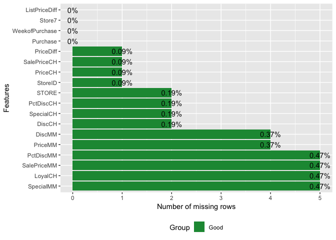
There are 40 missing observations in the data set.In this exploratory analysis we would simply delete these missing values. Imputing missing values would be discussed extensively in a later post.When the number of missing values is relative to the sample size is small in a data set, a basic approach to handling missing data is to delete them.
plot_missing(orangejuice)
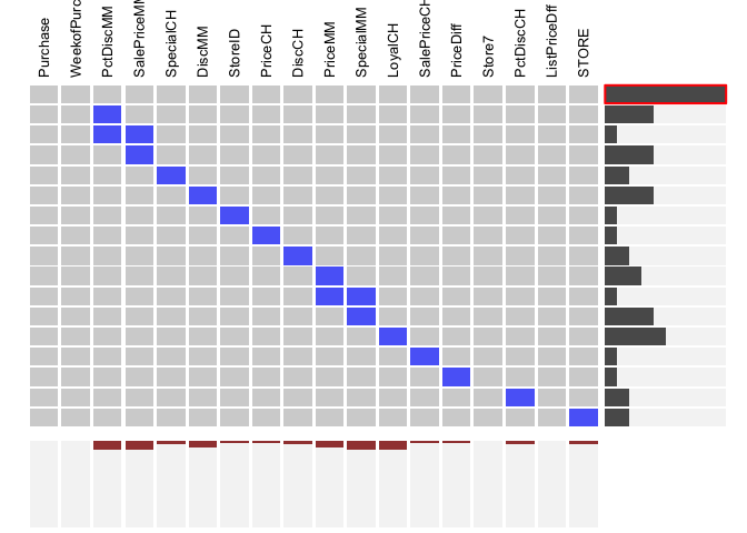
An alternate visualization approach is to use visna function from the extracat package.The columns represent the variables in the data and the rows the missing pattern.The blue cells represent cells of the variable with missing values.The proportion of missing values for each variable is shown by the bars vertically beneath cells.The right show the relative frequencies of patterns.
pacman::p_load(extracat)


extracat::visna(orangejuice, sort = "b", sort.method="optile", fr=100, pmax=0.05, s = 2)
library(VIM)
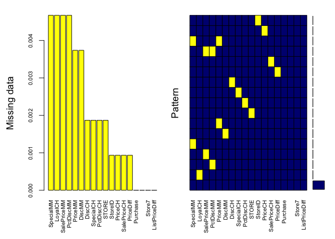
aggr(orangejuice , col=c('navyblue','yellow'),
numbers=TRUE, sortVars=TRUE,
labels=names(orangejuice), cex.axis=.7,
gap=3, ylab=c("Missing data","Pattern"))
##
##  Variables sorted by number of missings:
##        Variable        Count
##       SpecialMM 0.0046728972
##         LoyalCH 0.0046728972
##     SalePriceMM 0.0046728972
##       PctDiscMM 0.0046728972
##         PriceMM 0.0037383178
##          DiscMM 0.0037383178
##          DiscCH 0.0018691589
##       SpecialCH 0.0018691589
##       PctDiscCH 0.0018691589
##           STORE 0.0018691589
##         StoreID 0.0009345794
##         PriceCH 0.0009345794
##     SalePriceCH 0.0009345794
##       PriceDiff 0.0009345794
##        Purchase 0.0000000000
##  WeekofPurchase 0.0000000000
##          Store7 0.0000000000
##   ListPriceDiff 0.0000000000
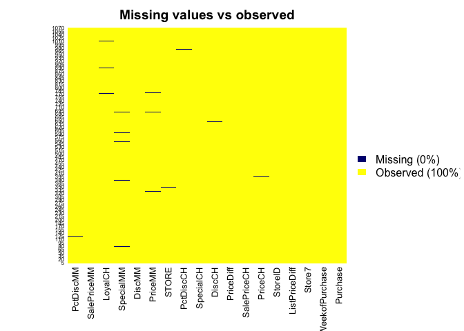
library(Amelia)
missmap(orangejuice, main = "Missing values vs observed",col=c('navyblue','yellow'),y.cex=0.5)
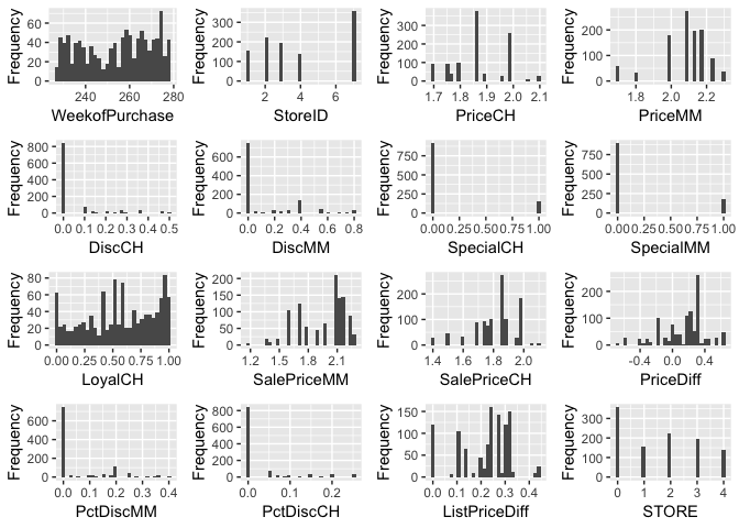
plot_histogram(orangejuice)
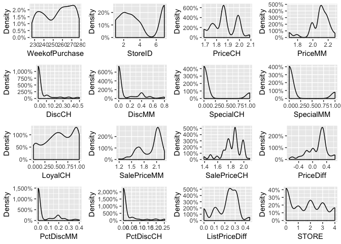
plot_density(orangejuice)
plot_bar(orangejuice)
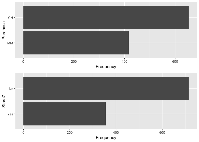
Purchases made at store store 7 is lower than other stores whereas more customers purchased Citrus Hill than Minute Maid Orange Juice
Multivariate Analysis
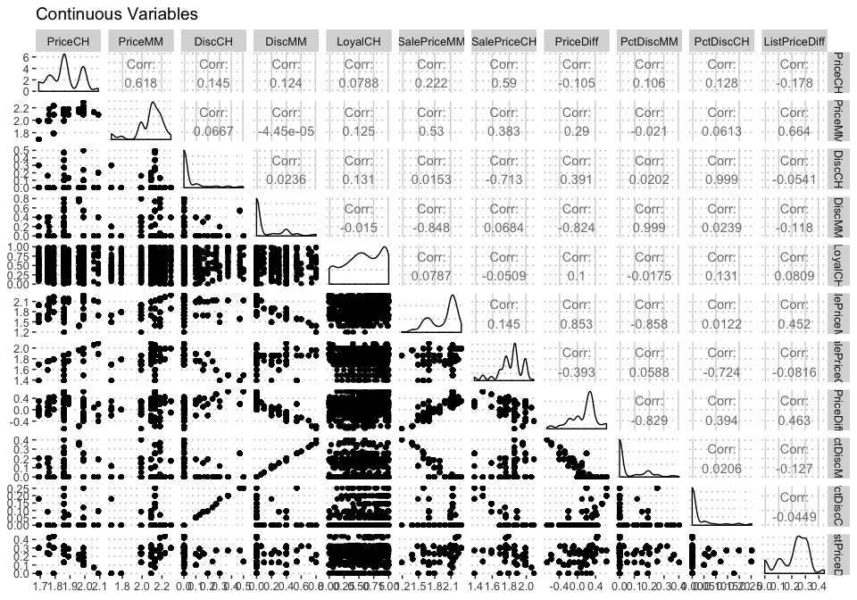
Multivariate analysis include examining the correlation structure between variables in the dataset and also the bivariate relationship between the response variable and each predictor variable.
pacman::p_load(GGally)

na.omit(orangejuice)%>%select_if(is.double)%>%ggpairs(  title = "Continuous Variables")
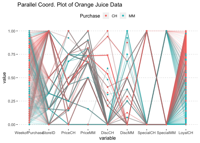
Multiple continuous variables can be visualized by Parallel Coordinate Plots (PCP). Each vertical axis represents a column variable in the data and the observations are drawn as lines connecting its value on the corresponding vertical axes. The ggplot extension GGally package has the ggparcoord function which can be used for PCP plots in R. High values for Week of purchase corresponds with stores with low ID numbers. Low values for Indicator of special on MM corresponds with higher customer loyalty
#p_ <- GGally::print_if_interactive

# this time, color by diamond cut
p <- ggparcoord(data = na.omit(orangejuice), columns = c(2:10), groupColumn = "Purchase", title = "Parallel Coord. Plot of Orange Juice Data",scale = "uniminmax", boxplot = FALSE, mapping = ggplot2::aes(size = 1),showPoints = TRUE,alpha = .05,)+
  #scale_fill_viridis(discrete = T)+

    scale_fill_manual(values=c("#B9DE28FF" , "#D1E11CFF" ))+
   ggplot2::scale_size_identity()
#p_(p)
p
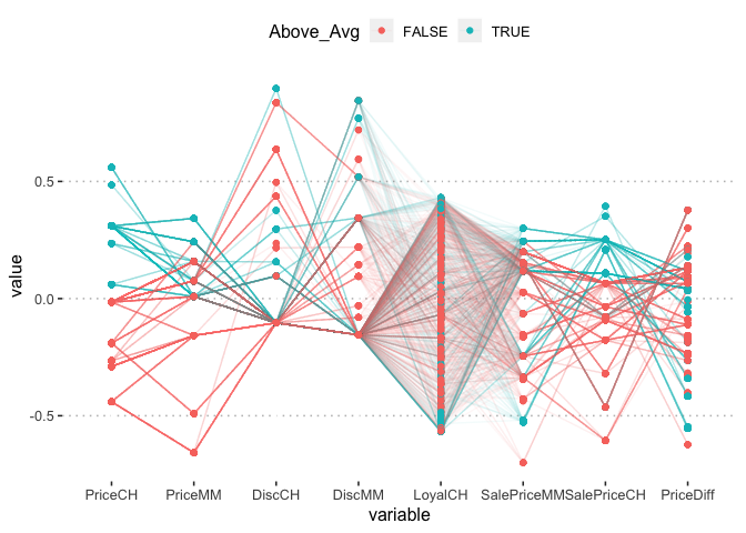
na.omit(orangejuice)%>%select_if(is.double)%>%
  mutate(Above_Avg = PriceCH > mean(PriceCH)) %>%
  GGally::ggparcoord(showPoints = TRUE,

    alpha = .05,
    scale = "center",
    columns = 1:8,
    groupColumn = "Above_Avg"
    )
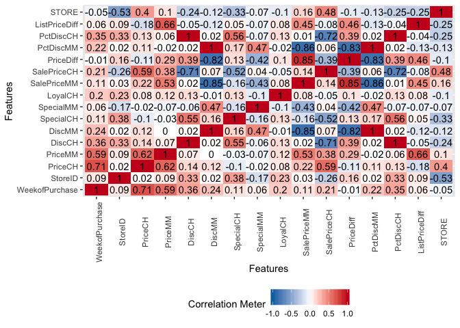
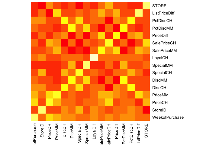
Correlation between numeric variables can also be visualized by a heatmap. Heatmaps can identify clusters with strong correlation among variables. The correlation matrix between the variables can be visualized neatly on a heatmap. e the correlation matrix and visualize this matrix with a heatmap. Deep points represent low correlations whereas light yellow represents strong correlations. There exist strong correlations among variable pairs such as (WeekofPurchase, Price) ,( PctDisc, SalePrice )for both CH and MM, ( ListPriceDiff, PriceMM) etc.
plot_correlation(na.omit(orangejuice),type = "continuous",theme_config = list(legend.position = "bottom", axis.text.x =
  element_text(angle = 90)))
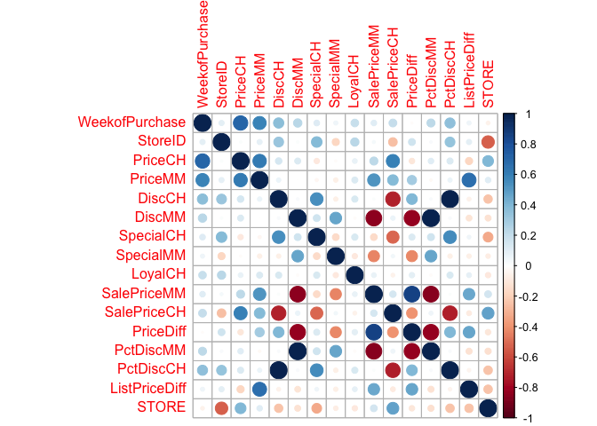
The corrplot function can also equivalently plot the correlatio between variables in a dataset as shown below:
pacman::p_load(plotly,corrr,RColorBrewer,corrplot)


na.omit(orangejuice)%>%select_if(is.numeric)%>%cor()%>%corrplot::corrplot()
#Equivalently
#na.omit(orangejuice)%>%select_if(is.numeric)%>%cor()%>%
#  corrplot.mixed(upper = "color", tl.col = "black")
na.omit(orangejuice)%>%
  select_if(is.numeric) %>%
  cor() %>%
  heatmap(Rowv = NA, Colv = NA, scale = "column")
An interactive heatmap can be easily plotted courtesy the d3heatmap package.
pacman::p_load(d3heatmap)

na.omit(orangejuice)%>%
  select_if(is.numeric) %>%
  cor() %>%
d3heatmap(colors = "Blues", scale = "col",
          dendrogram = "row", k_row = 3)

ggsave("/Users/nanaakwasiabayieboateng/Documents/memphisclassesbooks/DataMiningscience/ExploratoryDataAnalysis/d3heatmap.pdf")
library(devtools)

#install_github("easyGgplot2", "kassambara")


pacman::p_load(ggalt,gridExtra,scales,kassambara,easyGgplot2)


p1<-ggplot(orangejuice, aes(x=SalePriceCH, fill=Purchase)) + geom_bkde(alpha=0.5)
p2<-ggplot(orangejuice, aes(x=SalePriceMM, fill=Purchase)) + geom_bkde(alpha=0.5)


# Multiple graphs on the same page
easyGgplot2::ggplot2.multiplot(p1,p2, cols=2)
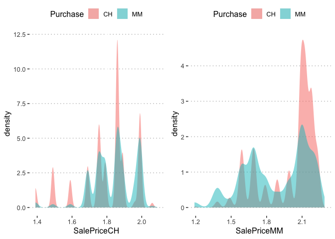
The sale price for both purchased Citrus Hill and Minute Maid Orange Juice is multimodal and the Citrus Hill has a higher sale price.
The skimr and mlr packages have functions that conveniently summaeizes a dataset and present the output in a tabular form.
skimmed <-skim_to_wide(orangejuice)
skimmed%>%
  kable() %>%
  kable_styling()
| type | variable | missing | complete | n | min | max | empty | n_unique | mean | sd | p0 | p25 | p50 | p75 | p100 | hist |
|---|---|---|---|---|---|---|---|---|---|---|---|---|---|---|---|---|
| character | Purchase | 0 | 1070 | 1070 | 2 | 2 | 0 | 2 | NA | NA | NA | NA | NA | NA | NA | NA |
| character | Store7 | 0 | 1070 | 1070 | 2 | 3 | 0 | 2 | NA | NA | NA | NA | NA | NA | NA | NA |
| integer | SpecialCH | 2 | 1068 | 1070 | NA | NA | NA | NA | 0.15 | 0.35 | 0 | 0 | 0 | 0 | 1 | ▇▁▁▁▁▁▁▂ |
| integer | SpecialMM | 5 | 1065 | 1070 | NA | NA | NA | NA | 0.16 | 0.37 | 0 | 0 | 0 | 0 | 1 | ▇▁▁▁▁▁▁▂ |
| integer | STORE | 2 | 1068 | 1070 | NA | NA | NA | NA | 1.63 | 1.43 | 0 | 0 | 2 | 3 | 4 | ▇▃▁▅▁▅▁▃ |
| integer | StoreID | 1 | 1069 | 1070 | NA | NA | NA | NA | 3.96 | 2.31 | 1 | 2 | 3 | 7 | 7 | ▃▅▅▃▁▁▁▇ |
| integer | WeekofPurchase | 0 | 1070 | 1070 | NA | NA | NA | NA | 254.38 | 15.56 | 227 | 240 | 257 | 268 | 278 | ▆▅▅▃▅▇▆▇ |
| numeric | DiscCH | 2 | 1068 | 1070 | NA | NA | NA | NA | 0.052 | 0.12 | 0 | 0 | 0 | 0 | 0.5 | ▇▁▁▁▁▁▁▁ |
| numeric | DiscMM | 4 | 1066 | 1070 | NA | NA | NA | NA | 0.12 | 0.21 | 0 | 0 | 0 | 0.23 | 0.8 | ▇▁▁▂▁▁▁▁ |
| numeric | ListPriceDiff | 0 | 1070 | 1070 | NA | NA | NA | NA | 0.22 | 0.11 | 0 | 0.14 | 0.24 | 0.3 | 0.44 | ▂▂▂▂▇▆▁▁ |
| numeric | LoyalCH | 5 | 1065 | 1070 | NA | NA | NA | NA | 0.57 | 0.31 | 1.1e-05 | 0.32 | 0.6 | 0.85 | 1 | ▅▂▃▃▆▃▃▇ |
| numeric | PctDiscCH | 2 | 1068 | 1070 | NA | NA | NA | NA | 0.027 | 0.062 | 0 | 0 | 0 | 0 | 0.25 | ▇▁▁▁▁▁▁▁ |
| numeric | PctDiscMM | 5 | 1065 | 1070 | NA | NA | NA | NA | 0.059 | 0.1 | 0 | 0 | 0 | 0.11 | 0.4 | ▇▁▁▂▁▁▁▁ |
| numeric | PriceCH | 1 | 1069 | 1070 | NA | NA | NA | NA | 1.87 | 0.1 | 1.69 | 1.79 | 1.86 | 1.99 | 2.09 | ▂▅▁▇▁▁▅▁ |
| numeric | PriceDiff | 1 | 1069 | 1070 | NA | NA | NA | NA | 0.15 | 0.27 | -0.67 | 0 | 0.23 | 0.32 | 0.64 | ▁▁▂▂▃▇▃▂ |
| numeric | PriceMM | 4 | 1066 | 1070 | NA | NA | NA | NA | 2.09 | 0.13 | 1.69 | 1.99 | 2.09 | 2.18 | 2.29 | ▁▁▁▃▁▇▃▂ |
| numeric | SalePriceCH | 1 | 1069 | 1070 | NA | NA | NA | NA | 1.82 | 0.14 | 1.39 | 1.75 | 1.86 | 1.89 | 2.09 | ▁▁▁▂▆▇▅▁ |
| numeric | SalePriceMM | 5 | 1065 | 1070 | NA | NA | NA | NA | 1.96 | 0.25 | 1.19 | 1.69 | 2.09 | 2.13 | 2.29 | ▁▁▃▃▁▂▇▆ |
mlr::summarizeColumns(orangejuice)%>%
  kable() %>%
  kable_styling()
| name | type | na | mean | disp | median | mad | min | max | nlevs |
|---|---|---|---|---|---|---|---|---|---|
| Purchase | character | 0 | NA | 0.3897196 | NA | NA | 4.17e+02 | 653.000000 | 2 |
| WeekofPurchase | integer | 0 | 254.3813084 | 15.5582861 | 257.00 | 20.7564000 | 2.27e+02 | 278.000000 | 0 |
| StoreID | integer | 1 | 3.9569691 | 2.3081886 | 3.00 | 1.4826000 | 1.00e+00 | 7.000000 | 0 |
| PriceCH | numeric | 1 | 1.8674275 | 0.1020172 | 1.86 | 0.1482600 | 1.69e+00 | 2.090000 | 0 |
| PriceMM | numeric | 4 | 2.0850375 | 0.1344285 | 2.09 | 0.1334340 | 1.69e+00 | 2.290000 | 0 |
| DiscCH | numeric | 2 | 0.0519569 | 0.1175628 | 0.00 | 0.0000000 | 0.00e+00 | 0.500000 | 0 |
| DiscMM | numeric | 4 | 0.1234146 | 0.2141255 | 0.00 | 0.0000000 | 0.00e+00 | 0.800000 | 0 |
| SpecialCH | integer | 2 | 0.1470037 | 0.3542755 | 0.00 | 0.0000000 | 0.00e+00 | 1.000000 | 0 |
| SpecialMM | integer | 5 | 0.1624413 | 0.3690285 | 0.00 | 0.0000000 | 0.00e+00 | 1.000000 | 0 |
| LoyalCH | numeric | 5 | 0.5652030 | 0.3080704 | 0.60 | 0.3891084 | 1.10e-05 | 0.999947 | 0 |
| SalePriceMM | numeric | 5 | 1.9619343 | 0.2525100 | 2.09 | 0.1482600 | 1.19e+00 | 2.290000 | 0 |
| SalePriceCH | numeric | 1 | 1.8155192 | 0.1434442 | 1.86 | 0.1482600 | 1.39e+00 | 2.090000 | 0 |
| PriceDiff | numeric | 1 | 0.1463237 | 0.2716379 | 0.23 | 0.1482600 | -6.70e-01 | 0.640000 | 0 |
| Store7 | character | 0 | NA | 0.3327103 | NA | NA | 3.56e+02 | 714.000000 | 2 |
| PctDiscMM | numeric | 5 | 0.0593881 | 0.1018414 | 0.00 | 0.0000000 | 0.00e+00 | 0.402010 | 0 |
| PctDiscCH | numeric | 2 | 0.0273179 | 0.0622811 | 0.00 | 0.0000000 | 0.00e+00 | 0.252688 | 0 |
| ListPriceDiff | numeric | 0 | 0.2179907 | 0.1075354 | 0.24 | 0.0889560 | 0.00e+00 | 0.440000 | 0 |
| STORE | integer | 2 | 1.6282772 | 1.4304973 | 2.00 | 1.4826000 | 0.00e+00 | 4.000000 | 0 |
(spec_variables <- attr(orangejuice, "spec"))
## cols(
##   Purchase = col_character(),
##   WeekofPurchase = col_integer(),
##   StoreID = col_integer(),
##   PriceCH = col_double(),
##   PriceMM = col_double(),
##   DiscCH = col_double(),
##   DiscMM = col_double(),
##   SpecialCH = col_integer(),
##   SpecialMM = col_integer(),
##   LoyalCH = col_double(),
##   SalePriceMM = col_double(),
##   SalePriceCH = col_double(),
##   PriceDiff = col_double(),
##   Store7 = col_character(),
##   PctDiscMM = col_double(),
##   PctDiscCH = col_double(),
##   ListPriceDiff = col_double(),
##   STORE = col_integer()
## )
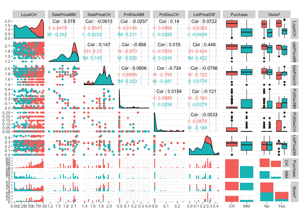
spec_variables<-c("LoyalCH", "SalePriceMM","SalePriceCH" ,"PctDiscMM","PctDiscCH","ListPriceDiff","Purchase","Store7")


spec_variable<-noquote(spec_variables)

pm<-ggpairs(orangejuice,spec_variable , title = "",mapping = aes(color = Purchase))+
  theme(legend.position = "top")

pm
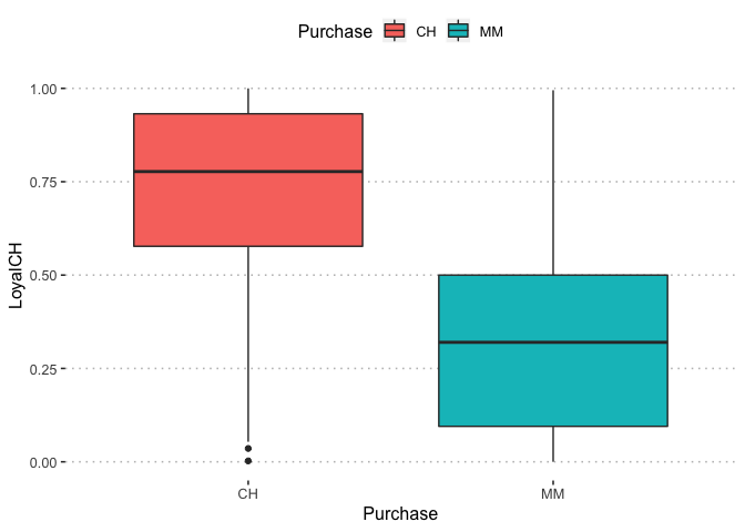
We can select one of plots above as follows:
pm[1,7]
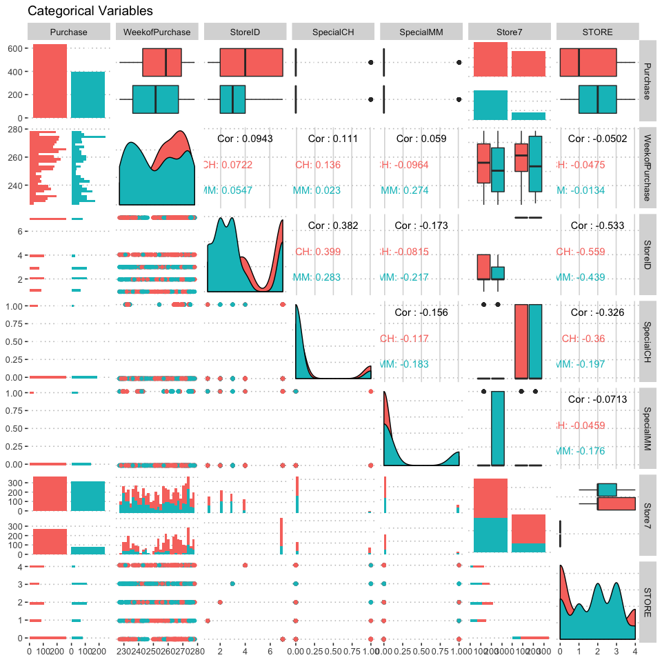
na.omit(orangejuice)%>% select_if(~!is.double(.x))%>%
  ggpairs( mapping = aes(color = Purchase) , title = "Categorical Variables")+
  theme(legend.position = "top")
#Equivalently

#na.omit(orangejuice)%>% select_if(funs(!is.double(.)))%>%
 # ggpairs(  title = "Categorical Variables")


#index=!sapply(na.omit(orangejuice), is.double)
#orange_numeric<-orangejuice[index==TRUE]
#orange_numeric%>%ggpairs(  title = "Categorical Variables")


#na.omit(orangejuice)%>%select_if(negate(is.double))%>%
#  ggpairs(  title = "Categorical Variables")
categorical_orange=na.omit(orangejuice)%>% select_if(~!is.double(.x))
continuous_orange=na.omit(orangejuice)%>% select_if(is.double)
categorical_orange<-noquote(names(categorical_orange))
continuous_orange<-noquote(names(continuous_orange))
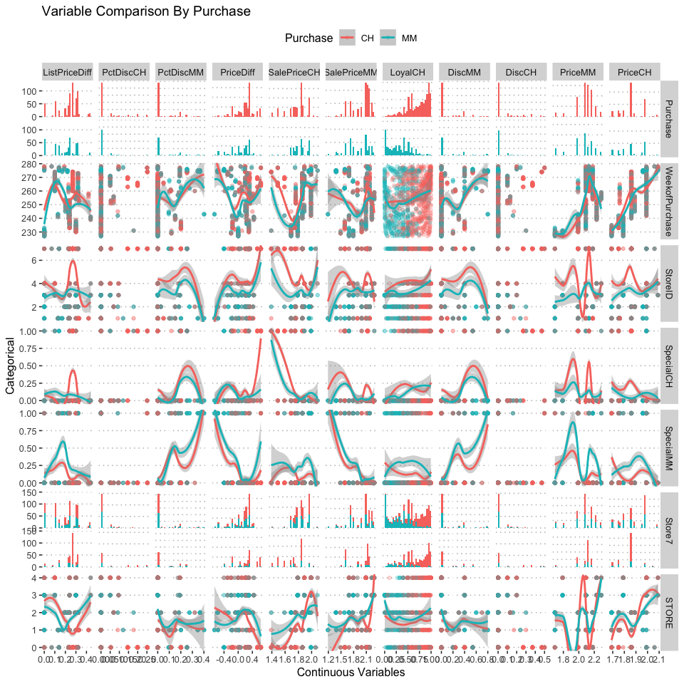
ggduo(
orangejuice, rev(continuous_orange), categorical_orange,
mapping = aes(color = Purchase),
types = list(continuous = wrap("smooth_loess", alpha = 0.25)),
showStrips = FALSE,
title = "Variable Comparison By Purchase",
xlab = "Continuous Variables",
ylab = "Categorical",
legend = c(5,2)
) +
theme(legend.position = "top")
#</body>